Lecture 10 - Databases and SQL

• 10.1 Introduction to SQL

• 10.2 Using SQLite with Python

• 10.3 Create a New Table

• 10.4 Database Example

• 10.5 Querying Databases with SELECT

• 10.6 Sorting Data with ORDER BY

• 10.7 Filtering Data

• 10.8 Conditional Expressions

• 10.9 Joining Multiple Tables

• 10.10 Return Data Statistics

• 10.11 Grouping Data

• 10.12 Modifying Data

• 10.13 Working with Tables

• 10.14 Constraints

• 10.15 Subqueries

• 10.16 Connect to an Existing Database

• References

10.1 Introduction to SQL

SQL (Structured Query Language) is a programming language designed for managing data in Relational Data Base Management Systems (RDBMS), or for stream processing in Relational Data Stream Management Systems (RDSMS). A relational database is a database that stores related information across multiple tables, and allows to query information in more than one table at the same time. Within a table, the data is organized in a tabular format with rows and columns.

SQL was initially developed in 1970, and since then different companies and vendors implemented SQL in their products with some variations. To bring greater conformity in the variants of SQL, the American National Standards Institute (ANSI) published the first SQL standard in 1986. The standard has been updated every few years since then.

Today, there are several variants of SQL for database management systems available, some of which were developed by companies such as IBM and Oracle, as well as there are variants developed by communities, such as MySQL, PostgreSQL, SQLite, MariaDB, SnowflakeSQL, etc. Although these variants of SQL have certain differences, they are based on the basic SQL syntax, and are quite similar.

The main advantages of SQL include standardized syntax (since all relational database systems have an SQL query interpreter built-in), and is easy-to-understand due to using English-like commands and functions.

Relational Databases

Relational databases store information in multiple tables, which allows to work with more complex data, and have flexibility in the way the data is organized. An example is shown in the next figure, where a database is shown that is used for managing the HR data of a small business.

This database has seven tables:

• Jobs table stores data related to job title and salary range.

• Employees table stores the data of employees.

• Dependents table stores the employee’s dependents.

• Departments table stores department data.

• Regions table stores the data of regions such as Asia, Europe, America, Middle East, and Africa.

• Countries table stores the data of countries where the company is doing business.

• Locations table stores the location of the departments of the company.

Each table contains many records with rows and columns (similar to an Excel spreadsheet), and the records have relationships across the tables. Using multiple tables in a relational database allows us to avoid duplication of information, in comparison to using a single table to store all information. Also, it provides flexibility in how we work with the data. To establish relationships between the records in different tables we need to use an ID or identifier for each employee. The identifier for each employee, or in general for each record (row) in a relational database, is referred to as primary key. For instance, each employee can be assigned an ID value (such as employee 162), and each table would have an ID column (primary key column) to establish the relationship with the other tables in the database, indicated with an asterisk in the tables.

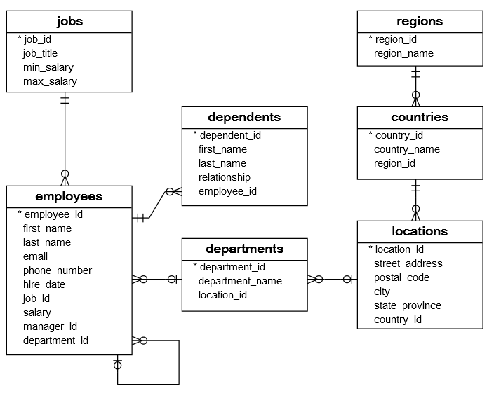Figure source: Reference [1].

SQL for Data Science

SQL is a very important tool for data scientists, data analysts, developers, and database administrators. In particular, as many companies become data-driven, SQL becomes an essential tool for handling data stored in databases and performing various data analytics operations, such as calculating data statistics, updating records, removing duplicate columns, calculating correlations between records, and similar.

SQL versus Pandas

SQL has similarities with the Pandas library, as it offers similar functionality to Pandas, which includes data manipulation over rows and columns, data merging, grouping, dealing with missing values, and similar. However, Pandas is not a relational database management library, but it is a data frame library.

Still, Pandas offers additional functions and flexibility for handling and manipulating tabular data, and many users download databases to their local machine, and afterward use Pandas for data processing, rather than using SQL to process the data on the server.

The benefits of using SQL over Pandas can depend on the task. Several considerations include:

• In the case of a large database of information (e.g., GigaBytes of data), downloading the database to the local machine to be processed by Pandas may be slow or infeasible. Pandas is more suitable for processing small to medium size databases in Python.

• Even if the user can download the data on the local machine for processing with Pandas, it may be required to apply some level of preprocessing or organizing the data on the server using SQL.

• Some tasks can require that the data processing is done in the existing database. Also, when the tasks require fast data retrieval and processing, SQL can be more efficient than Pandas.

SQLite

In this lecture, we will use SQLite which implements a self-contained, serverless SQL database engine. SQLite is lightweight in terms of setup and required recourses. Unlike most other SQL variants, SQLite does not have a separate server process, and it reads and writes directly to disk files. That is, it does not use the client/server model. Because it has no server managing access to it, SQLite is not suitable in multiuser environments where multiple people can simultaneously edit files.

10.2 Using SQLite with Python

To demonstrate the use of SQLite with Python, in this lecture we will use magic commands in Jupyter Notebook. Magic commands are special commands which are not valid Python code, but perform certain actions in a Jupyter Notebook. They begin with the % symbol.

The library ipython-sql offers the magic functions %sql and %%sql, which allow to connect to a database and use standard SQL commands in Jupyter Notebooks. To run ipython-sql on your computer, it needs to be installed (e.g., by using either conda install -c conda-forge ipython-sql or via pip install ipython-sql). If we run this notebook on Google Colab, ipython-sql comes preinstalled and there is no need to install it.

To load the ipython-sql library we will use %load_ext sql as in the next code. %load_ext is a magic command that loads an external package that can add new magic commands.

%load_ext sql

The magic command %sql is used to execute an SQL query that is contained in a single statement in a Jupyter notebook cell, and %%sql allows to execute an SQL query that is contained in multiple SQL statements in a single cell.

10.3 Create a New Table

To create a new table we will use the SQL command CREATE TABLE, as shown in the next cell. If the table already exists in the database, an error message will show up.

In order to establish a connection to the newly created table, we used %%sql sqlite:// in the cell below. If we wanted to create a new table in an existing database to which we have already established a connection, we could have used only the magic command %%sql.

SQL has many commands or keywords that have special meaning, such as SELECT, INSERT, DELETE, and these keywords cannot be used as names of tables, columns, or other objects.

To make SQL language more readable, it is a convention to write the SQL commands with uppercase letters, and the other variables and identifiers with lowercase letters. However, this is not required, as the SQL commands are not case-sensitive.

Let’s create a table called cars which has 3 columns: id, name, and price. In the cell below, we specify that the values of id and price columns are integers, denoted by the INTEGER keyword. The names in the name column have a TEXT type. We also specified with NOT NULL that the values should not be missing in the id and name columns, i.e., when we insert data into the table we have to specify the values for the NON NULL columns.

Each table can have only one PRIMARY KEY column that uniquely identifies each row in the table, and prevents from inserting duplicate rows in the table. For the table below we set PRIMARY KEY to the id column. It is not required to define a primary key, however, it is a good practice to do it for every table.

%%sql sqlite://
CREATE TABLE cars(
    id INTEGER NOT NULL PRIMARY KEY,
    name TEXT NOT NULL,
    price INTEGER);

Done.

[]

The table that we just created is empty, and to add data to the table we will use the INSERT statement. In each row we provide values for id, name, and price.

When using multiple statements in SQL, the statements in each line need to be separated with a semicolon ;. The last statement in a cell does not have to be followed by a semicolon.

Inline comments can be inserted by using two consecutive hyphens -- that comment the rest of the line, as shown in the second line of the next cell.

And also, comments that span multiple lines can be inserted by using the multiline C-style notation /* comment */ as in the last lines in the cell.

Note also that we used just the magic command %%sql in this cell, and we didn’t need to write %%sql sqlite:// as in the above cell. The reason is that in the above cell we used %%sql sqlite:// to establish a connection to the newly created table. Once a connection is established, we can use only %sql or %%sql to work with the table.

%%sql
INSERT INTO cars VALUES(1,'Audi',52642); --Two consecutive hyphens (--) comment the rest of the line
INSERT INTO cars VALUES(2,'Mercedes',57127);
INSERT INTO cars VALUES(3,'Skoda',9000);
INSERT INTO cars VALUES(4,'Volvo',29000);
INSERT INTO cars VALUES(5,'Bentley',350000);
INSERT INTO cars VALUES(6,'Citroen',21000);
INSERT INTO cars VALUES(7,'Hummer',41400);
INSERT INTO cars VALUES(8,'Volkswagen',21600);
/* A comment that spans
more than one line */

 * sqlite://
1 rows affected.
1 rows affected.
1 rows affected.
1 rows affected.
1 rows affected.
1 rows affected.
1 rows affected.
1 rows affected.
Done.

[]

We can display the table with the following code. Notice again that we used a single % in the magic command %sql, since we have only one line of code.

Note: If you get an error message when running this cell, install prettytable using pip install prettytable==3.5.0. If you don’t get any errors, then disregard this note

%sql SELECT * FROM cars

 * sqlite://
Done.

id	name	price
1	Audi	52642
2	Mercedes	57127
3	Skoda	9000
4	Volvo	29000
5	Bentley	350000
6	Citroen	21000
7	Hummer	41400
8	Volkswagen	21600

Another Example of Creating a Table

In the next simple example, we will create another table called writer, with columns FirstName, LastName, and Year.

%%sql sqlite://
CREATE TABLE writer(
    FirstName TEXT NOT NULL,
    LastName TEXT NOT NULL,
    Year INTEGER NOT NULL PRIMARY KEY);

Done.

[]

In the INSERT statement, we can also include the column names after the table name, as in writer (FirstName,LastName,Year). This is not required, but it can reduce errors in entering the values for each column.

%%sql
INSERT INTO writer (FirstName,LastName,Year) VALUES ('William', 'Shakespeare', 1616);
INSERT INTO writer (FirstName,LastName,Year) VALUES ('Lin', 'Han', 1996);
INSERT INTO writer (FirstName,LastName,Year) VALUES ('Peter', 'Brecht', 1978);

 * sqlite://
1 rows affected.
1 rows affected.
1 rows affected.

[]

%sql SELECT * FROM writer

 * sqlite://
Done.

FirstName	LastName	Year
William	Shakespeare	1616
Peter	Brecht	1978
Lin	Han	1996

10.4 Database Example

As an example of a database, let’s create a database that was shown in the above section, related to managing the HR data of a small business.

The cells below first create the tables (recall that the database has 7 tables), and afterward the information for each table is inserted.

%%sql sqlite://

CREATE TABLE regions (
    region_id INTEGER PRIMARY KEY AUTOINCREMENT NOT NULL,
    region_name TEXT NOT NULL);

CREATE TABLE countries (
    country_id TEXT NOT NULL,
    country_name TEXT NOT NULL,
    region_id INTEGER NOT NULL,
    PRIMARY KEY (country_id ASC),
    FOREIGN KEY (region_id) REFERENCES regions (region_id) ON DELETE CASCADE ON UPDATE CASCADE);

CREATE TABLE locations (
    location_id INTEGER PRIMARY KEY AUTOINCREMENT NOT NULL,
    street_address TEXT,
    postal_code TEXT,
    city text NOT NULL,
    state_province TEXT,
    country_id INTEGER NOT NULL,
    FOREIGN KEY (country_id) REFERENCES countries (country_id) ON DELETE CASCADE ON UPDATE CASCADE);

CREATE TABLE departments (
    department_id INTEGER PRIMARY KEY AUTOINCREMENT NOT NULL,
    department_name TEXT NOT NULL,
    location_id INTEGER NOT NULL,
    FOREIGN KEY (location_id) REFERENCES locations (location_id) ON DELETE CASCADE ON UPDATE CASCADE);

CREATE TABLE jobs (
    job_id INTEGER PRIMARY KEY AUTOINCREMENT NOT NULL,
    job_title TEXT NOT NULL,
    min_salary DOUBLE NOT NULL,
    max_salary DOUBLE NOT NULL);

CREATE TABLE employees (
    employee_id INTEGER PRIMARY KEY AUTOINCREMENT NOT NULL,
    first_name TEXT,
    last_name TEXT NOT NULL,
    email TEXT NOT NULL,
    phone_number TEXT,
    hire_date TEXT NOT NULL,
    job_id INTEGER NOT NULL,
    salary DOUBLE NOT NULL,
    manager_id INTEGER,
    department_id INTEGER NOT NULL,
    FOREIGN KEY (job_id) REFERENCES jobs (job_id) ON DELETE CASCADE ON UPDATE CASCADE,
    FOREIGN KEY (department_id) REFERENCES departments (department_id) ON DELETE CASCADE ON UPDATE CASCADE,
    FOREIGN KEY (manager_id) REFERENCES employees (employee_id) ON DELETE CASCADE ON UPDATE CASCADE);

CREATE TABLE dependents (
    dependent_id INTEGER PRIMARY KEY AUTOINCREMENT NOT NULL,
    first_name TEXT NOT NULL,
    last_name TEXT NOT NULL,
    relationship TEXT NOT NULL,
    employee_id INTEGER NOT NULL,
    FOREIGN KEY (employee_id) REFERENCES employees (employee_id) ON DELETE CASCADE ON UPDATE CASCADE);

Done.
Done.
Done.
Done.
Done.
Done.
Done.

[]

%%sql

/*Data for the table regions */
INSERT INTO regions(region_id,region_name) VALUES (1,'Europe');
INSERT INTO regions(region_id,region_name) VALUES (2,'Americas');
INSERT INTO regions(region_id,region_name) VALUES (3,'Asia');
INSERT INTO regions(region_id,region_name) VALUES (4,'Middle East and Africa');

/*Data for the table countries */
INSERT INTO countries(country_id,country_name,region_id) VALUES ('AR','Argentina',2);
INSERT INTO countries(country_id,country_name,region_id) VALUES ('AU','Australia',3);
INSERT INTO countries(country_id,country_name,region_id) VALUES ('BE','Belgium',1);
INSERT INTO countries(country_id,country_name,region_id) VALUES ('BR','Brazil',2);
INSERT INTO countries(country_id,country_name,region_id) VALUES ('CA','Canada',2);
INSERT INTO countries(country_id,country_name,region_id) VALUES ('CH','Switzerland',1);
INSERT INTO countries(country_id,country_name,region_id) VALUES ('CN','China',3);
INSERT INTO countries(country_id,country_name,region_id) VALUES ('DE','Germany',1);
INSERT INTO countries(country_id,country_name,region_id) VALUES ('DK','Denmark',1);
INSERT INTO countries(country_id,country_name,region_id) VALUES ('EG','Egypt',4);
INSERT INTO countries(country_id,country_name,region_id) VALUES ('FR','France',1);
INSERT INTO countries(country_id,country_name,region_id) VALUES ('HK','HongKong',3);
INSERT INTO countries(country_id,country_name,region_id) VALUES ('IL','Israel',4);
INSERT INTO countries(country_id,country_name,region_id) VALUES ('IN','India',3);
INSERT INTO countries(country_id,country_name,region_id) VALUES ('IT','Italy',1);
INSERT INTO countries(country_id,country_name,region_id) VALUES ('JP','Japan',3);
INSERT INTO countries(country_id,country_name,region_id) VALUES ('KW','Kuwait',4);
INSERT INTO countries(country_id,country_name,region_id) VALUES ('MX','Mexico',2);
INSERT INTO countries(country_id,country_name,region_id) VALUES ('NG','Nigeria',4);
INSERT INTO countries(country_id,country_name,region_id) VALUES ('NL','Netherlands',1);
INSERT INTO countries(country_id,country_name,region_id) VALUES ('SG','Singapore',3);
INSERT INTO countries(country_id,country_name,region_id) VALUES ('UK','United Kingdom',1);
INSERT INTO countries(country_id,country_name,region_id) VALUES ('US','United States of America',2);
INSERT INTO countries(country_id,country_name,region_id) VALUES ('ZM','Zambia',4);
INSERT INTO countries(country_id,country_name,region_id) VALUES ('ZW','Zimbabwe',4);

/*Data for the table locations */
INSERT INTO locations(location_id,street_address,postal_code,city,state_province,country_id) VALUES (1400,'2014 Jabberwocky Rd','26192','Southlake','Texas','US');
INSERT INTO locations(location_id,street_address,postal_code,city,state_province,country_id) VALUES (1500,'2011 Interiors Blvd','99236','South San Francisco','California','US');
INSERT INTO locations(location_id,street_address,postal_code,city,state_province,country_id) VALUES (1700,'2004 Charade Rd','98199','Seattle','Washington','US');
INSERT INTO locations(location_id,street_address,postal_code,city,state_province,country_id) VALUES (1800,'147 Spadina Ave','M5V 2L7','Toronto','Ontario','CA');
INSERT INTO locations(location_id,street_address,postal_code,city,state_province,country_id) VALUES (2400,'8204 Arthur St',NULL,'London',NULL,'UK');
INSERT INTO locations(location_id,street_address,postal_code,city,state_province,country_id) VALUES (2500,'Magdalen Centre, The Oxford Science Park','OX9 9ZB','Oxford','Oxford','UK');
INSERT INTO locations(location_id,street_address,postal_code,city,state_province,country_id) VALUES (2700,'Schwanthalerstr. 7031','80925','Munich','Bavaria','DE');

/*Data for the table jobs */
INSERT INTO jobs(job_id,job_title,min_salary,max_salary) VALUES (1,'Public Accountant',4200.00,9000.00);
INSERT INTO jobs(job_id,job_title,min_salary,max_salary) VALUES (2,'Accounting Manager',8200.00,16000.00);
INSERT INTO jobs(job_id,job_title,min_salary,max_salary) VALUES (3,'Administration Assistant',3000.00,6000.00);
INSERT INTO jobs(job_id,job_title,min_salary,max_salary) VALUES (4,'President',20000.00,40000.00);
INSERT INTO jobs(job_id,job_title,min_salary,max_salary) VALUES (5,'Administration Vice President',15000.00,30000.00);
INSERT INTO jobs(job_id,job_title,min_salary,max_salary) VALUES (6,'Accountant',4200.00,9000.00);
INSERT INTO jobs(job_id,job_title,min_salary,max_salary) VALUES (7,'Finance Manager',8200.00,16000.00);
INSERT INTO jobs(job_id,job_title,min_salary,max_salary) VALUES (8,'Human Resources Representative',4000.00,9000.00);
INSERT INTO jobs(job_id,job_title,min_salary,max_salary) VALUES (9,'Programmer',4000.00,10000.00);
INSERT INTO jobs(job_id,job_title,min_salary,max_salary) VALUES (10,'Marketing Manager',9000.00,15000.00);
INSERT INTO jobs(job_id,job_title,min_salary,max_salary) VALUES (11,'Marketing Representative',4000.00,9000.00);
INSERT INTO jobs(job_id,job_title,min_salary,max_salary) VALUES (12,'Public Relations Representative',4500.00,10500.00);
INSERT INTO jobs(job_id,job_title,min_salary,max_salary) VALUES (13,'Purchasing Clerk',2500.00,5500.00);
INSERT INTO jobs(job_id,job_title,min_salary,max_salary) VALUES (14,'Purchasing Manager',8000.00,15000.00);
INSERT INTO jobs(job_id,job_title,min_salary,max_salary) VALUES (15,'Sales Manager',10000.00,20000.00);
INSERT INTO jobs(job_id,job_title,min_salary,max_salary) VALUES (16,'Sales Representative',6000.00,12000.00);
INSERT INTO jobs(job_id,job_title,min_salary,max_salary) VALUES (17,'Shipping Clerk',2500.00,5500.00);
INSERT INTO jobs(job_id,job_title,min_salary,max_salary) VALUES (18,'Stock Clerk',2000.00,5000.00);
INSERT INTO jobs(job_id,job_title,min_salary,max_salary) VALUES (19,'Stock Manager',5500.00,8500.00);

/*Data for the table departments */
INSERT INTO departments(department_id,department_name,location_id) VALUES (1,'Administration',1700);
INSERT INTO departments(department_id,department_name,location_id) VALUES (2,'Marketing',1800);
INSERT INTO departments(department_id,department_name,location_id) VALUES (3,'Purchasing',1700);
INSERT INTO departments(department_id,department_name,location_id) VALUES (4,'Human Resources',2400);
INSERT INTO departments(department_id,department_name,location_id) VALUES (5,'Shipping',1500);
INSERT INTO departments(department_id,department_name,location_id) VALUES (6,'IT',1400);
INSERT INTO departments(department_id,department_name,location_id) VALUES (7,'Public Relations',2700);
INSERT INTO departments(department_id,department_name,location_id) VALUES (8,'Sales',2500);
INSERT INTO departments(department_id,department_name,location_id) VALUES (9,'Executive',1700);
INSERT INTO departments(department_id,department_name,location_id) VALUES (10,'Finance',1700);
INSERT INTO departments(department_id,department_name,location_id) VALUES (11,'Accounting',1700);

/*Data for the table employees */
INSERT INTO employees(employee_id,first_name,last_name,email,phone_number,hire_date,job_id,salary,manager_id,department_id) VALUES (100,'Steven','King','steven.king@sqltutorial.org','515.123.4567','1987-06-17',4,24000.00,NULL,9);
INSERT INTO employees(employee_id,first_name,last_name,email,phone_number,hire_date,job_id,salary,manager_id,department_id) VALUES (101,'Neena','Kochhar','neena.kochhar@sqltutorial.org','515.123.4568','1989-09-21',5,17000.00,100,9);
INSERT INTO employees(employee_id,first_name,last_name,email,phone_number,hire_date,job_id,salary,manager_id,department_id) VALUES (102,'Lex','De Haan','lex.de haan@sqltutorial.org','515.123.4569','1993-01-13',5,17000.00,100,9);
INSERT INTO employees(employee_id,first_name,last_name,email,phone_number,hire_date,job_id,salary,manager_id,department_id) VALUES (103,'Alexander','Hunold','alexander.hunold@sqltutorial.org','590.423.4567','1990-01-03',9,9000.00,102,6);
INSERT INTO employees(employee_id,first_name,last_name,email,phone_number,hire_date,job_id,salary,manager_id,department_id) VALUES (104,'Bruce','Ernst','bruce.ernst@sqltutorial.org','590.423.4568','1991-05-21',9,6000.00,103,6);
INSERT INTO employees(employee_id,first_name,last_name,email,phone_number,hire_date,job_id,salary,manager_id,department_id) VALUES (105,'David','Austin','david.austin@sqltutorial.org','590.423.4569','1997-06-25',9,4800.00,103,6);
INSERT INTO employees(employee_id,first_name,last_name,email,phone_number,hire_date,job_id,salary,manager_id,department_id) VALUES (106,'Valli','Pataballa','valli.pataballa@sqltutorial.org','590.423.4560','1998-02-05',9,4800.00,103,6);
INSERT INTO employees(employee_id,first_name,last_name,email,phone_number,hire_date,job_id,salary,manager_id,department_id) VALUES (107,'Diana','Lorentz','diana.lorentz@sqltutorial.org','590.423.5567','1999-02-07',9,4200.00,103,6);
INSERT INTO employees(employee_id,first_name,last_name,email,phone_number,hire_date,job_id,salary,manager_id,department_id) VALUES (108,'Nancy','Greenberg','nancy.greenberg@sqltutorial.org','515.124.4569','1994-08-17',7,12000.00,101,10);
INSERT INTO employees(employee_id,first_name,last_name,email,phone_number,hire_date,job_id,salary,manager_id,department_id) VALUES (109,'Daniel','Faviet','daniel.faviet@sqltutorial.org','515.124.4169','1994-08-16',6,9000.00,108,10);
INSERT INTO employees(employee_id,first_name,last_name,email,phone_number,hire_date,job_id,salary,manager_id,department_id) VALUES (110,'John','Chen','john.chen@sqltutorial.org','515.124.4269','1997-09-28',6,8200.00,108,10);
INSERT INTO employees(employee_id,first_name,last_name,email,phone_number,hire_date,job_id,salary,manager_id,department_id) VALUES (111,'Ismael','Sciarra','ismael.sciarra@sqltutorial.org','515.124.4369','1997-09-30',6,7700.00,108,10);
INSERT INTO employees(employee_id,first_name,last_name,email,phone_number,hire_date,job_id,salary,manager_id,department_id) VALUES (112,'Jose Manuel','Urman','jose manuel.urman@sqltutorial.org','515.124.4469','1998-03-07',6,7800.00,108,10);
INSERT INTO employees(employee_id,first_name,last_name,email,phone_number,hire_date,job_id,salary,manager_id,department_id) VALUES (113,'Luis','Popp','luis.popp@sqltutorial.org','515.124.4567','1999-12-07',6,6900.00,108,10);
INSERT INTO employees(employee_id,first_name,last_name,email,phone_number,hire_date,job_id,salary,manager_id,department_id) VALUES (114,'Den','Raphaely','den.raphaely@sqltutorial.org','515.127.4561','1994-12-07',14,11000.00,100,3);
INSERT INTO employees(employee_id,first_name,last_name,email,phone_number,hire_date,job_id,salary,manager_id,department_id) VALUES (115,'Alexander','Khoo','alexander.khoo@sqltutorial.org','515.127.4562','1995-05-18',13,3100.00,114,3);
INSERT INTO employees(employee_id,first_name,last_name,email,phone_number,hire_date,job_id,salary,manager_id,department_id) VALUES (116,'Shelli','Baida','shelli.baida@sqltutorial.org','515.127.4563','1997-12-24',13,2900.00,114,3);
INSERT INTO employees(employee_id,first_name,last_name,email,phone_number,hire_date,job_id,salary,manager_id,department_id) VALUES (117,'Sigal','Tobias','sigal.tobias@sqltutorial.org','515.127.4564','1997-07-24',13,2800.00,114,3);
INSERT INTO employees(employee_id,first_name,last_name,email,phone_number,hire_date,job_id,salary,manager_id,department_id) VALUES (118,'Guy','Himuro','guy.himuro@sqltutorial.org','515.127.4565','1998-11-15',13,2600.00,114,3);
INSERT INTO employees(employee_id,first_name,last_name,email,phone_number,hire_date,job_id,salary,manager_id,department_id) VALUES (119,'Karen','Colmenares','karen.colmenares@sqltutorial.org','515.127.4566','1999-08-10',13,2500.00,114,3);
INSERT INTO employees(employee_id,first_name,last_name,email,phone_number,hire_date,job_id,salary,manager_id,department_id) VALUES (120,'Matthew','Weiss','matthew.weiss@sqltutorial.org','650.123.1234','1996-07-18',19,8000.00,100,5);
INSERT INTO employees(employee_id,first_name,last_name,email,phone_number,hire_date,job_id,salary,manager_id,department_id) VALUES (121,'Adam','Fripp','adam.fripp@sqltutorial.org','650.123.2234','1997-04-10',19,8200.00,100,5);
INSERT INTO employees(employee_id,first_name,last_name,email,phone_number,hire_date,job_id,salary,manager_id,department_id) VALUES (122,'Payam','Kaufling','payam.kaufling@sqltutorial.org','650.123.3234','1995-05-01',19,7900.00,100,5);
INSERT INTO employees(employee_id,first_name,last_name,email,phone_number,hire_date,job_id,salary,manager_id,department_id) VALUES (123,'Shanta','Vollman','shanta.vollman@sqltutorial.org','650.123.4234','1997-10-10',19,6500.00,100,5);
INSERT INTO employees(employee_id,first_name,last_name,email,phone_number,hire_date,job_id,salary,manager_id,department_id) VALUES (126,'Irene','Mikkilineni','irene.mikkilineni@sqltutorial.org','650.124.1224','1998-09-28',18,2700.00,120,5);
INSERT INTO employees(employee_id,first_name,last_name,email,phone_number,hire_date,job_id,salary,manager_id,department_id) VALUES (145,'John','Russell','john.russell@sqltutorial.org',NULL,'1996-10-01',15,14000.00,100,8);
INSERT INTO employees(employee_id,first_name,last_name,email,phone_number,hire_date,job_id,salary,manager_id,department_id) VALUES (146,'Karen','Partners','karen.partners@sqltutorial.org',NULL,'1997-01-05',15,13500.00,100,8);
INSERT INTO employees(employee_id,first_name,last_name,email,phone_number,hire_date,job_id,salary,manager_id,department_id) VALUES (176,'Jonathon','Taylor','jonathon.taylor@sqltutorial.org',NULL,'1998-03-24',16,8600.00,100,8);
INSERT INTO employees(employee_id,first_name,last_name,email,phone_number,hire_date,job_id,salary,manager_id,department_id) VALUES (177,'Jack','Livingston','jack.livingston@sqltutorial.org',NULL,'1998-04-23',16,8400.00,100,8);
INSERT INTO employees(employee_id,first_name,last_name,email,phone_number,hire_date,job_id,salary,manager_id,department_id) VALUES (178,'Kimberely','Grant','kimberely.grant@sqltutorial.org',NULL,'1999-05-24',16,7000.00,100,8);
INSERT INTO employees(employee_id,first_name,last_name,email,phone_number,hire_date,job_id,salary,manager_id,department_id) VALUES (179,'Charles','Johnson','charles.johnson@sqltutorial.org',NULL,'2000-01-04',16,6200.00,100,8);
INSERT INTO employees(employee_id,first_name,last_name,email,phone_number,hire_date,job_id,salary,manager_id,department_id) VALUES (192,'Sarah','Bell','sarah.bell@sqltutorial.org','650.501.1876','1996-02-04',17,4000.00,123,5);
INSERT INTO employees(employee_id,first_name,last_name,email,phone_number,hire_date,job_id,salary,manager_id,department_id) VALUES (193,'Britney','Everett','britney.everett@sqltutorial.org','650.501.2876','1997-03-03',17,3900.00,123,5);
INSERT INTO employees(employee_id,first_name,last_name,email,phone_number,hire_date,job_id,salary,manager_id,department_id) VALUES (200,'Jennifer','Whalen','jennifer.whalen@sqltutorial.org','515.123.4444','1987-09-17',3,4400.00,101,1);
INSERT INTO employees(employee_id,first_name,last_name,email,phone_number,hire_date,job_id,salary,manager_id,department_id) VALUES (201,'Michael','Hartstein','michael.hartstein@sqltutorial.org','515.123.5555','1996-02-17',10,13000.00,100,2);
INSERT INTO employees(employee_id,first_name,last_name,email,phone_number,hire_date,job_id,salary,manager_id,department_id) VALUES (202,'Pat','Fay','pat.fay@sqltutorial.org','603.123.6666','1997-08-17',11,6000.00,201,2);
INSERT INTO employees(employee_id,first_name,last_name,email,phone_number,hire_date,job_id,salary,manager_id,department_id) VALUES (203,'Susan','Mavris','susan.mavris@sqltutorial.org','515.123.7777','1994-06-07',8,6500.00,101,4);
INSERT INTO employees(employee_id,first_name,last_name,email,phone_number,hire_date,job_id,salary,manager_id,department_id) VALUES (204,'Hermann','Baer','hermann.baer@sqltutorial.org','515.123.8888','1994-06-07',12,10000.00,101,7);
INSERT INTO employees(employee_id,first_name,last_name,email,phone_number,hire_date,job_id,salary,manager_id,department_id) VALUES (205,'Shelley','Higgins','shelley.higgins@sqltutorial.org','515.123.8080','1994-06-07',2,12000.00,101,11);
INSERT INTO employees(employee_id,first_name,last_name,email,phone_number,hire_date,job_id,salary,manager_id,department_id) VALUES (206,'William','Gietz','william.gietz@sqltutorial.org','515.123.8181','1994-06-07',1,8300.00,205,11);

/*Data for the table dependents */
INSERT INTO dependents(dependent_id,first_name,last_name,relationship,employee_id) VALUES (1,'Penelope','Gietz','Child',206);
INSERT INTO dependents(dependent_id,first_name,last_name,relationship,employee_id) VALUES (2,'Nick','Higgins','Child',205);
INSERT INTO dependents(dependent_id,first_name,last_name,relationship,employee_id) VALUES (3,'Ed','Whalen','Child',200);
INSERT INTO dependents(dependent_id,first_name,last_name,relationship,employee_id) VALUES (4,'Jennifer','King','Child',100);
INSERT INTO dependents(dependent_id,first_name,last_name,relationship,employee_id) VALUES (5,'Johnny','Kochhar','Child',101);
INSERT INTO dependents(dependent_id,first_name,last_name,relationship,employee_id) VALUES (6,'Bette','De Haan','Child',102);
INSERT INTO dependents(dependent_id,first_name,last_name,relationship,employee_id) VALUES (7,'Grace','Faviet','Child',109);
INSERT INTO dependents(dependent_id,first_name,last_name,relationship,employee_id) VALUES (8,'Matthew','Chen','Child',110);
INSERT INTO dependents(dependent_id,first_name,last_name,relationship,employee_id) VALUES (9,'Joe','Sciarra','Child',111);
INSERT INTO dependents(dependent_id,first_name,last_name,relationship,employee_id) VALUES (10,'Christian','Urman','Child',112);
INSERT INTO dependents(dependent_id,first_name,last_name,relationship,employee_id) VALUES (11,'Zero','Popp','Child',113);
INSERT INTO dependents(dependent_id,first_name,last_name,relationship,employee_id) VALUES (12,'Karl','Greenberg','Child',108);
INSERT INTO dependents(dependent_id,first_name,last_name,relationship,employee_id) VALUES (13,'Uma','Mavris','Child',203);
INSERT INTO dependents(dependent_id,first_name,last_name,relationship,employee_id) VALUES (14,'Vivien','Hunold','Child',103);
INSERT INTO dependents(dependent_id,first_name,last_name,relationship,employee_id) VALUES (15,'Cuba','Ernst','Child',104);
INSERT INTO dependents(dependent_id,first_name,last_name,relationship,employee_id) VALUES (16,'Fred','Austin','Child',105);
INSERT INTO dependents(dependent_id,first_name,last_name,relationship,employee_id) VALUES (17,'Helen','Pataballa','Child',106);
INSERT INTO dependents(dependent_id,first_name,last_name,relationship,employee_id) VALUES (18,'Dan','Lorentz','Child',107);
INSERT INTO dependents(dependent_id,first_name,last_name,relationship,employee_id) VALUES (19,'Bob','Hartstein','Child',201);
INSERT INTO dependents(dependent_id,first_name,last_name,relationship,employee_id) VALUES (20,'Lucille','Fay','Child',202);
INSERT INTO dependents(dependent_id,first_name,last_name,relationship,employee_id) VALUES (21,'Kirsten','Baer','Child',204);
INSERT INTO dependents(dependent_id,first_name,last_name,relationship,employee_id) VALUES (22,'Elvis','Khoo','Child',115);
INSERT INTO dependents(dependent_id,first_name,last_name,relationship,employee_id) VALUES (23,'Sandra','Baida','Child',116);
INSERT INTO dependents(dependent_id,first_name,last_name,relationship,employee_id) VALUES (24,'Cameron','Tobias','Child',117);
INSERT INTO dependents(dependent_id,first_name,last_name,relationship,employee_id) VALUES (25,'Kevin','Himuro','Child',118);
INSERT INTO dependents(dependent_id,first_name,last_name,relationship,employee_id) VALUES (26,'Rip','Colmenares','Child',119);
INSERT INTO dependents(dependent_id,first_name,last_name,relationship,employee_id) VALUES (27,'Julia','Raphaely','Child',114);
INSERT INTO dependents(dependent_id,first_name,last_name,relationship,employee_id) VALUES (28,'Woody','Russell','Child',145);
INSERT INTO dependents(dependent_id,first_name,last_name,relationship,employee_id) VALUES (29,'Alec','Partners','Child',146);
INSERT INTO dependents(dependent_id,first_name,last_name,relationship,employee_id) VALUES (30,'Sandra','Taylor','Child',176);

 * sqlite://
1 rows affected.
1 rows affected.
1 rows affected.
1 rows affected.
1 rows affected.
1 rows affected.
1 rows affected.
1 rows affected.
1 rows affected.
1 rows affected.
1 rows affected.
1 rows affected.
1 rows affected.
1 rows affected.
1 rows affected.
1 rows affected.
1 rows affected.
1 rows affected.
1 rows affected.
1 rows affected.
1 rows affected.
1 rows affected.
1 rows affected.
1 rows affected.
1 rows affected.
1 rows affected.
1 rows affected.
1 rows affected.
1 rows affected.
1 rows affected.
1 rows affected.
1 rows affected.
1 rows affected.
1 rows affected.
1 rows affected.
1 rows affected.
1 rows affected.
1 rows affected.
1 rows affected.
1 rows affected.
1 rows affected.
1 rows affected.
1 rows affected.
1 rows affected.
1 rows affected.
1 rows affected.
1 rows affected.
1 rows affected.
1 rows affected.
1 rows affected.
1 rows affected.
1 rows affected.
1 rows affected.
1 rows affected.
1 rows affected.
1 rows affected.
1 rows affected.
1 rows affected.
1 rows affected.
1 rows affected.
1 rows affected.
1 rows affected.
1 rows affected.
1 rows affected.
1 rows affected.
1 rows affected.
1 rows affected.
1 rows affected.
1 rows affected.
1 rows affected.
1 rows affected.
1 rows affected.
1 rows affected.
1 rows affected.
1 rows affected.
1 rows affected.
1 rows affected.
1 rows affected.
1 rows affected.
1 rows affected.
1 rows affected.
1 rows affected.
1 rows affected.
1 rows affected.
1 rows affected.
1 rows affected.
1 rows affected.
1 rows affected.
1 rows affected.
1 rows affected.
1 rows affected.
1 rows affected.
1 rows affected.
1 rows affected.
1 rows affected.
1 rows affected.
1 rows affected.
1 rows affected.
1 rows affected.
1 rows affected.
1 rows affected.
1 rows affected.
1 rows affected.
1 rows affected.
1 rows affected.
1 rows affected.
1 rows affected.
1 rows affected.
1 rows affected.
1 rows affected.
1 rows affected.
1 rows affected.
1 rows affected.
1 rows affected.
1 rows affected.
1 rows affected.
1 rows affected.
1 rows affected.
1 rows affected.
1 rows affected.
1 rows affected.
1 rows affected.
1 rows affected.
1 rows affected.
1 rows affected.
1 rows affected.
1 rows affected.
1 rows affected.
1 rows affected.
1 rows affected.
1 rows affected.
1 rows affected.
1 rows affected.
1 rows affected.
1 rows affected.
1 rows affected.

[]

10.5 Querying Databases with SELECT

The most common SQL task is to retrieve data from one or more tables. The data is returned in the form of a result table, called result set. This is accomplished with the SELECT statement, which has the following general syntax.

SELECT
    column1, column2, columnN
FROM
    table_name

For example, in the next cell we retrieved the columns employee_id, first_name, last_name, hire_date from the employees table. When the statement is evaluated, the database system first evaluates the FROM clause and the SELECT clause afterward. I.e., from the table named employees select the listed columns.

%%sql
SELECT
    employee_id, first_name, last_name, hire_date
FROM
    employees

 * sqlite://
Done.

employee_id	first_name	last_name	hire_date
100	Steven	King	1987-06-17
101	Neena	Kochhar	1989-09-21
102	Lex	De Haan	1993-01-13
103	Alexander	Hunold	1990-01-03
104	Bruce	Ernst	1991-05-21
105	David	Austin	1997-06-25
106	Valli	Pataballa	1998-02-05
107	Diana	Lorentz	1999-02-07
108	Nancy	Greenberg	1994-08-17
109	Daniel	Faviet	1994-08-16
110	John	Chen	1997-09-28
111	Ismael	Sciarra	1997-09-30
112	Jose Manuel	Urman	1998-03-07
113	Luis	Popp	1999-12-07
114	Den	Raphaely	1994-12-07
115	Alexander	Khoo	1995-05-18
116	Shelli	Baida	1997-12-24
117	Sigal	Tobias	1997-07-24
118	Guy	Himuro	1998-11-15
119	Karen	Colmenares	1999-08-10
120	Matthew	Weiss	1996-07-18
121	Adam	Fripp	1997-04-10
122	Payam	Kaufling	1995-05-01
123	Shanta	Vollman	1997-10-10
126	Irene	Mikkilineni	1998-09-28
145	John	Russell	1996-10-01
146	Karen	Partners	1997-01-05
176	Jonathon	Taylor	1998-03-24
177	Jack	Livingston	1998-04-23
178	Kimberely	Grant	1999-05-24
179	Charles	Johnson	2000-01-04
192	Sarah	Bell	1996-02-04
193	Britney	Everett	1997-03-03
200	Jennifer	Whalen	1987-09-17
201	Michael	Hartstein	1996-02-17
202	Pat	Fay	1997-08-17
203	Susan	Mavris	1994-06-07
204	Hermann	Baer	1994-06-07
205	Shelley	Higgins	1994-06-07
206	William	Gietz	1994-06-07

If we want to query all columns in a table we can use the asterisk operator * instead of the columns names.

%sql SELECT * FROM employees

 * sqlite://
Done.

employee_id	first_name	last_name	email	phone_number	hire_date	job_id	salary	manager_id	department_id
100	Steven	King	steven.king@sqltutorial.org	515.123.4567	1987-06-17	4	24000.0	None	9
101	Neena	Kochhar	neena.kochhar@sqltutorial.org	515.123.4568	1989-09-21	5	17000.0	100	9
102	Lex	De Haan	lex.de haan@sqltutorial.org	515.123.4569	1993-01-13	5	17000.0	100	9
103	Alexander	Hunold	alexander.hunold@sqltutorial.org	590.423.4567	1990-01-03	9	9000.0	102	6
104	Bruce	Ernst	bruce.ernst@sqltutorial.org	590.423.4568	1991-05-21	9	6000.0	103	6
105	David	Austin	david.austin@sqltutorial.org	590.423.4569	1997-06-25	9	4800.0	103	6
106	Valli	Pataballa	valli.pataballa@sqltutorial.org	590.423.4560	1998-02-05	9	4800.0	103	6
107	Diana	Lorentz	diana.lorentz@sqltutorial.org	590.423.5567	1999-02-07	9	4200.0	103	6
108	Nancy	Greenberg	nancy.greenberg@sqltutorial.org	515.124.4569	1994-08-17	7	12000.0	101	10
109	Daniel	Faviet	daniel.faviet@sqltutorial.org	515.124.4169	1994-08-16	6	9000.0	108	10
110	John	Chen	john.chen@sqltutorial.org	515.124.4269	1997-09-28	6	8200.0	108	10
111	Ismael	Sciarra	ismael.sciarra@sqltutorial.org	515.124.4369	1997-09-30	6	7700.0	108	10
112	Jose Manuel	Urman	jose manuel.urman@sqltutorial.org	515.124.4469	1998-03-07	6	7800.0	108	10
113	Luis	Popp	luis.popp@sqltutorial.org	515.124.4567	1999-12-07	6	6900.0	108	10
114	Den	Raphaely	den.raphaely@sqltutorial.org	515.127.4561	1994-12-07	14	11000.0	100	3
115	Alexander	Khoo	alexander.khoo@sqltutorial.org	515.127.4562	1995-05-18	13	3100.0	114	3
116	Shelli	Baida	shelli.baida@sqltutorial.org	515.127.4563	1997-12-24	13	2900.0	114	3
117	Sigal	Tobias	sigal.tobias@sqltutorial.org	515.127.4564	1997-07-24	13	2800.0	114	3
118	Guy	Himuro	guy.himuro@sqltutorial.org	515.127.4565	1998-11-15	13	2600.0	114	3
119	Karen	Colmenares	karen.colmenares@sqltutorial.org	515.127.4566	1999-08-10	13	2500.0	114	3
120	Matthew	Weiss	matthew.weiss@sqltutorial.org	650.123.1234	1996-07-18	19	8000.0	100	5
121	Adam	Fripp	adam.fripp@sqltutorial.org	650.123.2234	1997-04-10	19	8200.0	100	5
122	Payam	Kaufling	payam.kaufling@sqltutorial.org	650.123.3234	1995-05-01	19	7900.0	100	5
123	Shanta	Vollman	shanta.vollman@sqltutorial.org	650.123.4234	1997-10-10	19	6500.0	100	5
126	Irene	Mikkilineni	irene.mikkilineni@sqltutorial.org	650.124.1224	1998-09-28	18	2700.0	120	5
145	John	Russell	john.russell@sqltutorial.org	None	1996-10-01	15	14000.0	100	8
146	Karen	Partners	karen.partners@sqltutorial.org	None	1997-01-05	15	13500.0	100	8
176	Jonathon	Taylor	jonathon.taylor@sqltutorial.org	None	1998-03-24	16	8600.0	100	8
177	Jack	Livingston	jack.livingston@sqltutorial.org	None	1998-04-23	16	8400.0	100	8
178	Kimberely	Grant	kimberely.grant@sqltutorial.org	None	1999-05-24	16	7000.0	100	8
179	Charles	Johnson	charles.johnson@sqltutorial.org	None	2000-01-04	16	6200.0	100	8
192	Sarah	Bell	sarah.bell@sqltutorial.org	650.501.1876	1996-02-04	17	4000.0	123	5
193	Britney	Everett	britney.everett@sqltutorial.org	650.501.2876	1997-03-03	17	3900.0	123	5
200	Jennifer	Whalen	jennifer.whalen@sqltutorial.org	515.123.4444	1987-09-17	3	4400.0	101	1
201	Michael	Hartstein	michael.hartstein@sqltutorial.org	515.123.5555	1996-02-17	10	13000.0	100	2
202	Pat	Fay	pat.fay@sqltutorial.org	603.123.6666	1997-08-17	11	6000.0	201	2
203	Susan	Mavris	susan.mavris@sqltutorial.org	515.123.7777	1994-06-07	8	6500.0	101	4
204	Hermann	Baer	hermann.baer@sqltutorial.org	515.123.8888	1994-06-07	12	10000.0	101	7
205	Shelley	Higgins	shelley.higgins@sqltutorial.org	515.123.8080	1994-06-07	2	12000.0	101	11
206	William	Gietz	william.gietz@sqltutorial.org	515.123.8181	1994-06-07	1	8300.0	205	11

List Tables in a Database

We can also use the SELECT statement to display a list of all tables in the current database. Every SQLite database has an sqlite_master table that defines the schema for the database. The schema refers to the organization or structure of a database, and includes various elements such as tables and columns names, the relationships between tables, the types of data, and constraints (primary keys and foreign keys) used in the database.

The following statement uses sqlite_master with the type field set to 'table' to return the names of all tables in the current database.

%sql SELECT name FROM sqlite_master WHERE type='table'

 * sqlite://
Done.

name
cars
writer
regions
sqlite_sequence
countries
locations
departments
jobs
employees
dependents

The next cell displays the entire sqlite_master table for the current database. It stores metadata about the tables and other objects in an SQLite database, and contains the columns type, name, tbl_name (the name of the table to which the object belongs), rootpage (the root page or page number of the object within the SQL database file), and sql (the SQL CREATE statement that was used to create the database). If the object is a table, the tbl_name is the same as the name in sqlite_master. Other types of objects in SQL include index, view, and trigger objects.

The sqlite_master table is automatically created and maintained by SQLite, and it is typically queried to inspect the schema of a database or retrieve information about its tables and other objects.

%sql SELECT * FROM sqlite_master

 * sqlite://
Done.

type	name	tbl_name	rootpage	sql
table	cars	cars	2	CREATE TABLE cars( id INTEGER NOT NULL PRIMARY KEY, name TEXT NOT NULL, price INTEGER)
table	writer	writer	3	CREATE TABLE writer( FirstName TEXT NOT NULL, LastName TEXT NOT NULL, Year INTEGER NOT NULL PRIMARY KEY)
table	regions	regions	4	CREATE TABLE regions ( region_id INTEGER PRIMARY KEY AUTOINCREMENT NOT NULL, region_name TEXT NOT NULL)
table	sqlite_sequence	sqlite_sequence	5	CREATE TABLE sqlite_sequence(name,seq)
table	countries	countries	6	CREATE TABLE countries ( country_id TEXT NOT NULL, country_name TEXT NOT NULL, region_id INTEGER NOT NULL, PRIMARY KEY (country_id ASC), FOREIGN KEY (region_id) REFERENCES regions (region_id) ON DELETE CASCADE ON UPDATE CASCADE)
index	sqlite_autoindex_countries_1	countries	7	None
table	locations	locations	8	CREATE TABLE locations ( location_id INTEGER PRIMARY KEY AUTOINCREMENT NOT NULL, street_address TEXT, postal_code TEXT, city text NOT NULL, state_province TEXT, country_id INTEGER NOT NULL, FOREIGN KEY (country_id) REFERENCES countries (country_id) ON DELETE CASCADE ON UPDATE CASCADE)
table	departments	departments	9	CREATE TABLE departments ( department_id INTEGER PRIMARY KEY AUTOINCREMENT NOT NULL, department_name TEXT NOT NULL, location_id INTEGER NOT NULL, FOREIGN KEY (location_id) REFERENCES locations (location_id) ON DELETE CASCADE ON UPDATE CASCADE)
table	jobs	jobs	10	CREATE TABLE jobs ( job_id INTEGER PRIMARY KEY AUTOINCREMENT NOT NULL, job_title TEXT NOT NULL, min_salary DOUBLE NOT NULL, max_salary DOUBLE NOT NULL)
table	employees	employees	11	CREATE TABLE employees ( employee_id INTEGER PRIMARY KEY AUTOINCREMENT NOT NULL, first_name TEXT, last_name TEXT NOT NULL, email TEXT NOT NULL, phone_number TEXT, hire_date TEXT NOT NULL, job_id INTEGER NOT NULL, salary DOUBLE NOT NULL, manager_id INTEGER, department_id INTEGER NOT NULL, FOREIGN KEY (job_id) REFERENCES jobs (job_id) ON DELETE CASCADE ON UPDATE CASCADE, FOREIGN KEY (department_id) REFERENCES departments (department_id) ON DELETE CASCADE ON UPDATE CASCADE, FOREIGN KEY (manager_id) REFERENCES employees (employee_id) ON DELETE CASCADE ON UPDATE CASCADE)
table	dependents	dependents	12	CREATE TABLE dependents ( dependent_id INTEGER PRIMARY KEY AUTOINCREMENT NOT NULL, first_name TEXT NOT NULL, last_name TEXT NOT NULL, relationship TEXT NOT NULL, employee_id INTEGER NOT NULL, FOREIGN KEY (employee_id) REFERENCES employees (employee_id) ON DELETE CASCADE ON UPDATE CASCADE)

For instance, we can use the following code to retrieve the CREATE statement for the table cars.

%sql SELECT sql FROM sqlite_master WHERE type='table' AND name='cars';

 * sqlite://
Done.

sql
CREATE TABLE cars( id INTEGER NOT NULL PRIMARY KEY, name TEXT NOT NULL, price INTEGER)

Perform Simple Calculations in SELECT Statements

We can use standard math operators such as +, *, /, % in SELECT statements to perform simple mathematical calculations. The following expression creates a new calculated field salary * 1.05 from the salary column and adds 5% to the salary of every employee. Specifically, the code does not create a new column in the table, but instead, it adds a new calculated field in the result set of the query.

%%sql
SELECT
    employee_id, first_name, salary, salary*1.05
FROM
    employees;

 * sqlite://
Done.

employee_id	first_name	salary	salary*1.05
100	Steven	24000.0	25200.0
101	Neena	17000.0	17850.0
102	Lex	17000.0	17850.0
103	Alexander	9000.0	9450.0
104	Bruce	6000.0	6300.0
105	David	4800.0	5040.0
106	Valli	4800.0	5040.0
107	Diana	4200.0	4410.0
108	Nancy	12000.0	12600.0
109	Daniel	9000.0	9450.0
110	John	8200.0	8610.0
111	Ismael	7700.0	8085.0
112	Jose Manuel	7800.0	8190.0
113	Luis	6900.0	7245.0
114	Den	11000.0	11550.0
115	Alexander	3100.0	3255.0
116	Shelli	2900.0	3045.0
117	Sigal	2800.0	2940.0
118	Guy	2600.0	2730.0
119	Karen	2500.0	2625.0
120	Matthew	8000.0	8400.0
121	Adam	8200.0	8610.0
122	Payam	7900.0	8295.0
123	Shanta	6500.0	6825.0
126	Irene	2700.0	2835.0
145	John	14000.0	14700.0
146	Karen	13500.0	14175.0
176	Jonathon	8600.0	9030.0
177	Jack	8400.0	8820.0
178	Kimberely	7000.0	7350.0
179	Charles	6200.0	6510.0
192	Sarah	4000.0	4200.0
193	Britney	3900.0	4095.0
200	Jennifer	4400.0	4620.0
201	Michael	13000.0	13650.0
202	Pat	6000.0	6300.0
203	Susan	6500.0	6825.0
204	Hermann	10000.0	10500.0
205	Shelley	12000.0	12600.0
206	William	8300.0	8715.0

We can use AS new_salary to assign a different name new_salary to the calculated field salary*1.05.

%%sql
SELECT
    employee_id, first_name, salary, salary*1.05 AS new_salary
FROM
    employees;

 * sqlite://
Done.

employee_id	first_name	salary	new_salary
100	Steven	24000.0	25200.0
101	Neena	17000.0	17850.0
102	Lex	17000.0	17850.0
103	Alexander	9000.0	9450.0
104	Bruce	6000.0	6300.0
105	David	4800.0	5040.0
106	Valli	4800.0	5040.0
107	Diana	4200.0	4410.0
108	Nancy	12000.0	12600.0
109	Daniel	9000.0	9450.0
110	John	8200.0	8610.0
111	Ismael	7700.0	8085.0
112	Jose Manuel	7800.0	8190.0
113	Luis	6900.0	7245.0
114	Den	11000.0	11550.0
115	Alexander	3100.0	3255.0
116	Shelli	2900.0	3045.0
117	Sigal	2800.0	2940.0
118	Guy	2600.0	2730.0
119	Karen	2500.0	2625.0
120	Matthew	8000.0	8400.0
121	Adam	8200.0	8610.0
122	Payam	7900.0	8295.0
123	Shanta	6500.0	6825.0
126	Irene	2700.0	2835.0
145	John	14000.0	14700.0
146	Karen	13500.0	14175.0
176	Jonathon	8600.0	9030.0
177	Jack	8400.0	8820.0
178	Kimberely	7000.0	7350.0
179	Charles	6200.0	6510.0
192	Sarah	4000.0	4200.0
193	Britney	3900.0	4095.0
200	Jennifer	4400.0	4620.0
201	Michael	13000.0	13650.0
202	Pat	6000.0	6300.0
203	Susan	6500.0	6825.0
204	Hermann	10000.0	10500.0
205	Shelley	12000.0	12600.0
206	William	8300.0	8715.0

10.6 Sorting Data with ORDER BY

The clause ORDER BY can be used within a SELECT statement to sort the returned rows.

The general syntax is:

SELECT
    column1, column2, columnN
FROM
    table_name
ORDER BY sort_expression [ASC | DESC];

The sort_expression specifies the sort criteria, whereas ASC or DESC indicates whether to sort the result set into ascending (default) or descending order.

The following example uses the clause ORDER BY to sort employees by first names in alphabetical order.

%%sql
SELECT
    employee_id, first_name, last_name, hire_date, salary
FROM
    employees
ORDER BY first_name;

 * sqlite://
Done.

employee_id	first_name	last_name	hire_date	salary
121	Adam	Fripp	1997-04-10	8200.0
103	Alexander	Hunold	1990-01-03	9000.0
115	Alexander	Khoo	1995-05-18	3100.0
193	Britney	Everett	1997-03-03	3900.0
104	Bruce	Ernst	1991-05-21	6000.0
179	Charles	Johnson	2000-01-04	6200.0
109	Daniel	Faviet	1994-08-16	9000.0
105	David	Austin	1997-06-25	4800.0
114	Den	Raphaely	1994-12-07	11000.0
107	Diana	Lorentz	1999-02-07	4200.0
118	Guy	Himuro	1998-11-15	2600.0
204	Hermann	Baer	1994-06-07	10000.0
126	Irene	Mikkilineni	1998-09-28	2700.0
111	Ismael	Sciarra	1997-09-30	7700.0
177	Jack	Livingston	1998-04-23	8400.0
200	Jennifer	Whalen	1987-09-17	4400.0
110	John	Chen	1997-09-28	8200.0
145	John	Russell	1996-10-01	14000.0
176	Jonathon	Taylor	1998-03-24	8600.0
112	Jose Manuel	Urman	1998-03-07	7800.0
119	Karen	Colmenares	1999-08-10	2500.0
146	Karen	Partners	1997-01-05	13500.0
178	Kimberely	Grant	1999-05-24	7000.0
102	Lex	De Haan	1993-01-13	17000.0
113	Luis	Popp	1999-12-07	6900.0
120	Matthew	Weiss	1996-07-18	8000.0
201	Michael	Hartstein	1996-02-17	13000.0
108	Nancy	Greenberg	1994-08-17	12000.0
101	Neena	Kochhar	1989-09-21	17000.0
202	Pat	Fay	1997-08-17	6000.0
122	Payam	Kaufling	1995-05-01	7900.0
192	Sarah	Bell	1996-02-04	4000.0
123	Shanta	Vollman	1997-10-10	6500.0
205	Shelley	Higgins	1994-06-07	12000.0
116	Shelli	Baida	1997-12-24	2900.0
117	Sigal	Tobias	1997-07-24	2800.0
100	Steven	King	1987-06-17	24000.0
203	Susan	Mavris	1994-06-07	6500.0
106	Valli	Pataballa	1998-02-05	4800.0
206	William	Gietz	1994-06-07	8300.0

The ORDER BY clause also allows using multiple expressions for sorting, separated by commas. In the following example ORDER BY is used to sort the employees by their first name in ascending order, and the employees who have the same first name are further sorted by their last name in descending order. E.g., check the sorting for the two employees with the name Alexander.

%%sql
SELECT
    employee_id, first_name, last_name, hire_date, salary
FROM
    employees
ORDER BY first_name, last_name DESC;

 * sqlite://
Done.

employee_id	first_name	last_name	hire_date	salary
121	Adam	Fripp	1997-04-10	8200.0
115	Alexander	Khoo	1995-05-18	3100.0
103	Alexander	Hunold	1990-01-03	9000.0
193	Britney	Everett	1997-03-03	3900.0
104	Bruce	Ernst	1991-05-21	6000.0
179	Charles	Johnson	2000-01-04	6200.0
109	Daniel	Faviet	1994-08-16	9000.0
105	David	Austin	1997-06-25	4800.0
114	Den	Raphaely	1994-12-07	11000.0
107	Diana	Lorentz	1999-02-07	4200.0
118	Guy	Himuro	1998-11-15	2600.0
204	Hermann	Baer	1994-06-07	10000.0
126	Irene	Mikkilineni	1998-09-28	2700.0
111	Ismael	Sciarra	1997-09-30	7700.0
177	Jack	Livingston	1998-04-23	8400.0
200	Jennifer	Whalen	1987-09-17	4400.0
145	John	Russell	1996-10-01	14000.0
110	John	Chen	1997-09-28	8200.0
176	Jonathon	Taylor	1998-03-24	8600.0
112	Jose Manuel	Urman	1998-03-07	7800.0
146	Karen	Partners	1997-01-05	13500.0
119	Karen	Colmenares	1999-08-10	2500.0
178	Kimberely	Grant	1999-05-24	7000.0
102	Lex	De Haan	1993-01-13	17000.0
113	Luis	Popp	1999-12-07	6900.0
120	Matthew	Weiss	1996-07-18	8000.0
201	Michael	Hartstein	1996-02-17	13000.0
108	Nancy	Greenberg	1994-08-17	12000.0
101	Neena	Kochhar	1989-09-21	17000.0
202	Pat	Fay	1997-08-17	6000.0
122	Payam	Kaufling	1995-05-01	7900.0
192	Sarah	Bell	1996-02-04	4000.0
123	Shanta	Vollman	1997-10-10	6500.0
205	Shelley	Higgins	1994-06-07	12000.0
116	Shelli	Baida	1997-12-24	2900.0
117	Sigal	Tobias	1997-07-24	2800.0
100	Steven	King	1987-06-17	24000.0
203	Susan	Mavris	1994-06-07	6500.0
106	Valli	Pataballa	1998-02-05	4800.0
206	William	Gietz	1994-06-07	8300.0

Similarly, we can use ORDER BY to sort columns with numerical data, or to sort by date as in the following cell.

%%sql
SELECT
    employee_id, first_name, last_name, hire_date, salary
FROM
    employees
ORDER BY hire_date;

 * sqlite://
Done.

employee_id	first_name	last_name	hire_date	salary
100	Steven	King	1987-06-17	24000.0
200	Jennifer	Whalen	1987-09-17	4400.0
101	Neena	Kochhar	1989-09-21	17000.0
103	Alexander	Hunold	1990-01-03	9000.0
104	Bruce	Ernst	1991-05-21	6000.0
102	Lex	De Haan	1993-01-13	17000.0
203	Susan	Mavris	1994-06-07	6500.0
204	Hermann	Baer	1994-06-07	10000.0
205	Shelley	Higgins	1994-06-07	12000.0
206	William	Gietz	1994-06-07	8300.0
109	Daniel	Faviet	1994-08-16	9000.0
108	Nancy	Greenberg	1994-08-17	12000.0
114	Den	Raphaely	1994-12-07	11000.0
122	Payam	Kaufling	1995-05-01	7900.0
115	Alexander	Khoo	1995-05-18	3100.0
192	Sarah	Bell	1996-02-04	4000.0
201	Michael	Hartstein	1996-02-17	13000.0
120	Matthew	Weiss	1996-07-18	8000.0
145	John	Russell	1996-10-01	14000.0
146	Karen	Partners	1997-01-05	13500.0
193	Britney	Everett	1997-03-03	3900.0
121	Adam	Fripp	1997-04-10	8200.0
105	David	Austin	1997-06-25	4800.0
117	Sigal	Tobias	1997-07-24	2800.0
202	Pat	Fay	1997-08-17	6000.0
110	John	Chen	1997-09-28	8200.0
111	Ismael	Sciarra	1997-09-30	7700.0
123	Shanta	Vollman	1997-10-10	6500.0
116	Shelli	Baida	1997-12-24	2900.0
106	Valli	Pataballa	1998-02-05	4800.0
112	Jose Manuel	Urman	1998-03-07	7800.0
176	Jonathon	Taylor	1998-03-24	8600.0
177	Jack	Livingston	1998-04-23	8400.0
126	Irene	Mikkilineni	1998-09-28	2700.0
118	Guy	Himuro	1998-11-15	2600.0
107	Diana	Lorentz	1999-02-07	4200.0
178	Kimberely	Grant	1999-05-24	7000.0
119	Karen	Colmenares	1999-08-10	2500.0
113	Luis	Popp	1999-12-07	6900.0
179	Charles	Johnson	2000-01-04	6200.0

10.7 Filtering Data

LIMIT

LIMIT is used to constrain the number of rows returned by a query, similar to the head() method in Pandas.

%%sql
SELECT
    employee_id, first_name, last_name, hire_date, salary
FROM
    employees
ORDER BY first_name
LIMIT 5;

 * sqlite://
Done.

employee_id	first_name	last_name	hire_date	salary
121	Adam	Fripp	1997-04-10	8200.0
103	Alexander	Hunold	1990-01-03	9000.0
115	Alexander	Khoo	1995-05-18	3100.0
193	Britney	Everett	1997-03-03	3900.0
104	Bruce	Ernst	1991-05-21	6000.0

It is also possible to include an OFFSET clause, which will skip rows before retrieving the data. E.g., in the next cell, the first 3 rows are skipped, and rows 4-8 are returned.

%%sql
SELECT
    employee_id, first_name, last_name, hire_date, salary
FROM
    employees
ORDER BY first_name
LIMIT 5
OFFSET 3;

 * sqlite://
Done.

employee_id	first_name	last_name	hire_date	salary
193	Britney	Everett	1997-03-03	3900.0
104	Bruce	Ernst	1991-05-21	6000.0
179	Charles	Johnson	2000-01-04	6200.0
109	Daniel	Faviet	1994-08-16	9000.0
105	David	Austin	1997-06-25	4800.0

DISTINCT

The DISTINCT clause allows to remove duplicate rows from the result set.

E.g., the next cell shows the first 15 rows of the salary columns, where some rows have the same value. In the cell afterward, DISTINCT is used to remove the rows with the same values for salary.

%%sql
SELECT
    salary
FROM
    employees
ORDER BY salary DESC
LIMIT 15;

 * sqlite://
Done.

salary
24000.0
17000.0
17000.0
14000.0
13500.0
13000.0
12000.0
12000.0
11000.0
10000.0
9000.0
9000.0
8600.0
8400.0
8300.0

%%sql
SELECT DISTINCT
    salary
FROM
    employees
ORDER BY salary DESC
LIMIT 15;

 * sqlite://
Done.

salary
24000.0
17000.0
14000.0
13500.0
13000.0
12000.0
11000.0
10000.0
9000.0
8600.0
8400.0
8300.0
8200.0
8000.0
7900.0

WHERE

The WHERE clause filters data based on specified conditions. For instance, return only the employees that have a salary greater than a certain value.

%%sql
SELECT
    employee_id, first_name, last_name,salary
FROM
    employees
WHERE salary > 9000
ORDER BY salary DESC;

 * sqlite://
Done.

employee_id	first_name	last_name	salary
100	Steven	King	24000.0
101	Neena	Kochhar	17000.0
102	Lex	De Haan	17000.0
145	John	Russell	14000.0
146	Karen	Partners	13500.0
201	Michael	Hartstein	13000.0
108	Nancy	Greenberg	12000.0
205	Shelley	Higgins	12000.0
114	Den	Raphaely	11000.0
204	Hermann	Baer	10000.0

Or, return the employees who work in the department 5.

%%sql
SELECT
    employee_id, first_name, last_name, salary, department_id
FROM
    employees
WHERE department_id = 5
ORDER BY first_name;

 * sqlite://
Done.

employee_id	first_name	last_name	salary	department_id
121	Adam	Fripp	8200.0	5
193	Britney	Everett	3900.0	5
126	Irene	Mikkilineni	2700.0	5
120	Matthew	Weiss	8000.0	5
122	Payam	Kaufling	7900.0	5
192	Sarah	Bell	4000.0	5
123	Shanta	Vollman	6500.0	5

Comparison Operators

To specify a condition, we can use the standard comparison operators, such as >, <, >=, <=, =, and note that <> can be used for 'not equal to'.

%%sql
SELECT
    employee_id, first_name, last_name, salary, department_id
FROM
    employees
WHERE department_id <> 5
ORDER BY first_name;

 * sqlite://
Done.

employee_id	first_name	last_name	salary	department_id
103	Alexander	Hunold	9000.0	6
115	Alexander	Khoo	3100.0	3
104	Bruce	Ernst	6000.0	6
179	Charles	Johnson	6200.0	8
109	Daniel	Faviet	9000.0	10
105	David	Austin	4800.0	6
114	Den	Raphaely	11000.0	3
107	Diana	Lorentz	4200.0	6
118	Guy	Himuro	2600.0	3
204	Hermann	Baer	10000.0	7
111	Ismael	Sciarra	7700.0	10
177	Jack	Livingston	8400.0	8
200	Jennifer	Whalen	4400.0	1
110	John	Chen	8200.0	10
145	John	Russell	14000.0	8
176	Jonathon	Taylor	8600.0	8
112	Jose Manuel	Urman	7800.0	10
119	Karen	Colmenares	2500.0	3
146	Karen	Partners	13500.0	8
178	Kimberely	Grant	7000.0	8
102	Lex	De Haan	17000.0	9
113	Luis	Popp	6900.0	10
201	Michael	Hartstein	13000.0	2
108	Nancy	Greenberg	12000.0	10
101	Neena	Kochhar	17000.0	9
202	Pat	Fay	6000.0	2
205	Shelley	Higgins	12000.0	11
116	Shelli	Baida	2900.0	3
117	Sigal	Tobias	2800.0	3
100	Steven	King	24000.0	9
203	Susan	Mavris	6500.0	4
106	Valli	Pataballa	4800.0	6
206	William	Gietz	8300.0	11

Logical Operators

We can also use logical operators to combine multiple conditions in the WHERE clause of an SQL statement. The following table contains the SQL logical operators.

Operator	Meaning
AND	Returns true if both expressions are true.
BETWEEN	Returns true if the operand is within a specified range.
OR	Returns true if either expression is true.
LIKE	Returns true if the operand matches a pattern.
IN	Returns true if the operand is equal to one of the values in a list.
NOT	Reverses the result of any other Boolean operator.

Following are several examples of using logical operators.

%%sql
SELECT
    first_name, last_name, salary
FROM
    employees
WHERE salary > 5000 AND salary < 7000
ORDER BY salary;

 * sqlite://
Done.

first_name	last_name	salary
Bruce	Ernst	6000.0
Pat	Fay	6000.0
Charles	Johnson	6200.0
Shanta	Vollman	6500.0
Susan	Mavris	6500.0
Luis	Popp	6900.0

%%sql
SELECT
    first_name, last_name, salary
FROM
    employees
WHERE salary BETWEEN 5000 AND 7000
ORDER BY salary;

 * sqlite://
Done.

first_name	last_name	salary
Bruce	Ernst	6000.0
Pat	Fay	6000.0
Charles	Johnson	6200.0
Shanta	Vollman	6500.0
Susan	Mavris	6500.0
Luis	Popp	6900.0
Kimberely	Grant	7000.0

%%sql
SELECT
    first_name, last_name, salary
FROM
    employees
WHERE salary = 6000 OR salary = 7000
ORDER BY salary;

 * sqlite://
Done.

first_name	last_name	salary
Bruce	Ernst	6000.0
Pat	Fay	6000.0
Kimberely	Grant	7000.0

Select employees with first names that start with jo by using the LIKE logical operator. The wildcard character % matches zero of more characters.

%%sql
SELECT
    employee_id, first_name, last_name
FROM
    employees
WHERE first_name LIKE 'jo%'
ORDER BY first_name;

 * sqlite://
Done.

employee_id	first_name	last_name
110	John	Chen
145	John	Russell
176	Jonathon	Taylor
112	Jose Manuel	Urman

Select employees with first names whose second character is h. The wildcard character _ matches exactly one character. Therefore, the first character in first_name can be any character.

%%sql
SELECT
    employee_id, first_name, last_name
FROM
    employees
WHERE
    first_name LIKE '_h%'
ORDER BY first_name;

 * sqlite://
Done.

employee_id	first_name	last_name
179	Charles	Johnson
123	Shanta	Vollman
205	Shelley	Higgins
116	Shelli	Baida

%%sql
SELECT
    first_name, last_name, department_id
FROM
    employees
WHERE department_id IN (8, 9)
ORDER BY department_id;

 * sqlite://
Done.

first_name	last_name	department_id
John	Russell	8
Karen	Partners	8
Jonathon	Taylor	8
Jack	Livingston	8
Kimberely	Grant	8
Charles	Johnson	8
Steven	King	9
Neena	Kochhar	9
Lex	De Haan	9

IS NULL Operator

To determine whether a row or column has missing or non-defined values, we can use the IS NULL operator.

For instance, to find all employees who do not have phone numbers, we use the IS NUL operator as follows.

%%sql
SELECT
    employee_id, first_name, last_name, phone_number
FROM
    employees
WHERE phone_number IS NULL

 * sqlite://
Done.

employee_id	first_name	last_name	phone_number
145	John	Russell	None
146	Karen	Partners	None
176	Jonathon	Taylor	None
177	Jack	Livingston	None
178	Kimberely	Grant	None
179	Charles	Johnson	None

10.8 Conditional Expressions

The CASE expression is used to add if-then-else logic to SQL statements, which allows to evaluate a list of conditions and returns one of the possible results.

In the next cell, the CASE expression returns the results Low, Average, or High based on the conditions regarding the salary. The results are collected in the evaluation column.

%%sql
SELECT
    first_name, last_name,
CASE WHEN salary < 3000 THEN 'Low'
     WHEN salary >= 3000 AND salary <= 5000 THEN 'Average'
     WHEN salary > 5000 THEN 'High'
END evaluation
FROM
    employees
LIMIT 15;

 * sqlite://
Done.

first_name	last_name	evaluation
Steven	King	High
Neena	Kochhar	High
Lex	De Haan	High
Alexander	Hunold	High
Bruce	Ernst	High
David	Austin	Average
Valli	Pataballa	Average
Diana	Lorentz	Average
Nancy	Greenberg	High
Daniel	Faviet	High
John	Chen	High
Ismael	Sciarra	High
Jose Manuel	Urman	High
Luis	Popp	High
Den	Raphaely	High

10.9 Joining Multiple Tables

SQL provides several ways to join tables, such as INNER JOIN, LEFT JOIN, RIGHT JOIN, FULL OUTER JOIN, and others.

INNER JOIN

INNER JOIN combines rows from two or more tables based on a related column between them. It retrieves only the rows that have matching values in both tables.

The syntax is:

SELECT
    column1, column2, ...
FROM
    table1
INNER JOIN table2 ON table1.columnX = table2.columnX;

It specifies to join table1 and table2 by matching values in columnX from table1 and columnX from table2, and returns column1, column2, ... from the joined tables.

Let’s show how we can use INNER JOIN, where for instance, we want to retrieve the list of employees who work in departments 1, 2, and 3, and we would like to list the names of the departments.

To do that, first we can notice that both the employees table and the departments table have a column department_id. Therefore, we can use the department_id column in the employees table as the foreign key column to link the employees to the departments table.

Let’s first display the employees who work in departments 1, 2, and 3 in the employees table to understand the data.

%%sql
SELECT
    first_name, last_name, department_id
FROM
    employees
WHERE department_id IN (1, 2, 3)
ORDER BY department_id;

 * sqlite://
Done.

first_name	last_name	department_id
Jennifer	Whalen	1
Michael	Hartstein	2
Pat	Fay	2
Den	Raphaely	3
Alexander	Khoo	3
Shelli	Baida	3
Sigal	Tobias	3
Guy	Himuro	3
Karen	Colmenares	3

We can also find the names of the departments in the departments table that have a department_id of 1, 2, and 3.

%%sql
SELECT
    department_id, department_name
FROM
    departments
WHERE department_id IN (1, 2, 3);

 * sqlite://
Done.

department_id	department_name
1	Administration
2	Marketing
3	Purchasing

Next, we join the employees and departments tables, and use INNER JOIN to match the department_id column in the two tables. For each row, if the condition departments.department_id = employees.department_id is satisfied, the combined row will include data from rows in both employees and departments tables in the result set.

%%sql
SELECT
    first_name, last_name, employees.department_id, departments.department_id, department_name
FROM
    employees
INNER JOIN departments ON employees.department_id = departments.department_id
WHERE employees.department_id IN (1, 2, 3);

 * sqlite://
Done.

first_name	last_name	department_id	department_id_1	department_name
Jennifer	Whalen	1	1	Administration
Michael	Hartstein	2	2	Marketing
Pat	Fay	2	2	Marketing
Den	Raphaely	3	3	Purchasing
Alexander	Khoo	3	3	Purchasing
Shelli	Baida	3	3	Purchasing
Sigal	Tobias	3	3	Purchasing
Guy	Himuro	3	3	Purchasing
Karen	Colmenares	3	3	Purchasing

Let’s look at one more example, where we used INNER JOIN to join three tables. Specifically, in the next cell we use one more INNER JOIN clause to join the tables employees and jobs using the job_id column, in order to retrieve the information about the job_title column from the jobs table.

%%sql
SELECT
    first_name, last_name, employees.department_id, departments.department_id,
    department_name, employees.job_id, jobs.job_id, job_title
FROM
    employees
INNER JOIN departments ON employees.department_id = departments.department_id
INNER JOIN jobs ON employees.job_id = jobs.job_id
WHERE employees.department_id IN (1, 2, 3);

 * sqlite://
Done.

first_name	last_name	department_id	department_id_1	department_name	job_id	job_id_1	job_title
Den	Raphaely	3	3	Purchasing	14	14	Purchasing Manager
Alexander	Khoo	3	3	Purchasing	13	13	Purchasing Clerk
Shelli	Baida	3	3	Purchasing	13	13	Purchasing Clerk
Sigal	Tobias	3	3	Purchasing	13	13	Purchasing Clerk
Guy	Himuro	3	3	Purchasing	13	13	Purchasing Clerk
Karen	Colmenares	3	3	Purchasing	13	13	Purchasing Clerk
Jennifer	Whalen	1	1	Administration	3	3	Administration Assistant
Michael	Hartstein	2	2	Marketing	10	10	Marketing Manager
Pat	Fay	2	2	Marketing	11	11	Marketing Representative

As we mentioned above, INNER JOIN retrieves only the rows that have matching values in both tables. This is shown in the figure below, which we already saw in the Pandas lecture. The table also shows other join operations.

Figure: Join Operations.

LEFT JOIN

LEFT JOIN (also referred to as LEFT OUTER JOIN) is similar to INNER JOIN, only it retrieves all rows from the left table in the JOIN clause and the matched rows from the right table.

The “left table” is the table that appears on the left side of the JOIN clause. It is considered the primary table, and its rows are the ones that we want to retrieve or work with primarily.

The “right table” is the table that appears on the right side of the JOIN clause. It is the secondary table, and we are typically interested in its data to complement or match with the data from the left table.

For instance, the countries table is shown below, with country_id column being the primary key. The following query returns columns for the countries US, UK, and China.

%%sql
SELECT
    country_id, country_name
FROM
    countries
WHERE country_id IN ('US', 'UK', 'CN');

 * sqlite://
Done.

country_id	country_name
CN	China
UK	United Kingdom
US	United States of America

Similarly, the locations table shown below has a country_id column as the foreign key. The query returns the locations located in the US, UK, and China.

%%sql
SELECT
    country_id, street_address, city
FROM
    locations
WHERE country_id IN ('US', 'UK', 'CN');

 * sqlite://
Done.

country_id	street_address	city
US	2014 Jabberwocky Rd	Southlake
US	2011 Interiors Blvd	South San Francisco
US	2004 Charade Rd	Seattle
UK	8204 Arthur St	London
UK	Magdalen Centre, The Oxford Science Park	Oxford

In the next cell, because we use the LEFT JOIN clause, all rows that satisfy the condition in the WHERE clause of the countries table are included in the result set.

For each row in the countries table, the LEFT JOIN clause finds the matching rows in the locations table. If at least one matching row is found, the database engine combines the data from columns of the matching rows in both tables.

In this case, there is no matching row found for the country China with the country_id of CN, and therefore, the row in the countries table is included in the result set and the rows in the locations table for China are filled with None values.

%%sql
SELECT
    country_name, countries.country_id, locations.country_id, street_address, city
FROM
    countries
LEFT JOIN locations ON countries.country_id = locations.country_id
WHERE countries.country_id IN ('US', 'UK', 'CN')

 * sqlite://
Done.

country_name	country_id	country_id_1	street_address	city
China	CN	None	None	None
United Kingdom	UK	UK	8204 Arthur St	London
United Kingdom	UK	UK	Magdalen Centre, The Oxford Science Park	Oxford
United States of America	US	US	2014 Jabberwocky Rd	Southlake
United States of America	US	US	2011 Interiors Blvd	South San Francisco
United States of America	US	US	2004 Charade Rd	Seattle

If we used LEFT JOIN for all rows in the countries table, the results would have been as in the following cell.

%%sql
SELECT
    country_name, countries.country_id, locations.country_id, street_address, city
FROM
    countries
LEFT JOIN locations ON countries.country_id = locations.country_id

 * sqlite://
Done.

country_name	country_id	country_id_1	street_address	city
Argentina	AR	None	None	None
Australia	AU	None	None	None
Belgium	BE	None	None	None
Brazil	BR	None	None	None
Canada	CA	CA	147 Spadina Ave	Toronto
Switzerland	CH	None	None	None
China	CN	None	None	None
Germany	DE	DE	Schwanthalerstr. 7031	Munich
Denmark	DK	None	None	None
Egypt	EG	None	None	None
France	FR	None	None	None
HongKong	HK	None	None	None
Israel	IL	None	None	None
India	IN	None	None	None
Italy	IT	None	None	None
Japan	JP	None	None	None
Kuwait	KW	None	None	None
Mexico	MX	None	None	None
Nigeria	NG	None	None	None
Netherlands	NL	None	None	None
Singapore	SG	None	None	None
United Kingdom	UK	UK	8204 Arthur St	London
United Kingdom	UK	UK	Magdalen Centre, The Oxford Science Park	Oxford
United States of America	US	US	2004 Charade Rd	Seattle
United States of America	US	US	2011 Interiors Blvd	South San Francisco
United States of America	US	US	2014 Jabberwocky Rd	Southlake
Zambia	ZM	None	None	None
Zimbabwe	ZW	None	None	None

LEFT JOIN is useful when we want to retrieve data from a primary table and include related information from a secondary table, but we don’t want to exclude records from the primary table if there are no matching rows in the secondary table.

And, because non-matching rows in the locations table are filled with the None values, we can apply the LEFT JOIN clause to find mismatched rows between the tables.

For example, to find the countries in the countries table that do not have any locations in the locations table, we can use the following query.

%%sql
SELECT
    country_name
FROM
    countries
LEFT JOIN locations ON countries.country_id = locations.country_id
WHERE locations.country_id IS NULL
ORDER BY country_name;

 * sqlite://
Done.

country_name
Argentina
Australia
Belgium
Brazil
China
Denmark
Egypt
France
HongKong
India
Israel
Italy
Japan
Kuwait
Mexico
Netherlands
Nigeria
Singapore
Switzerland
Zambia
Zimbabwe

RIGHT JOIN

By analogy, RIGHT JOIN (or RIGHT OUTER JOIN) returns all rows from the right table and the matched rows from the left table. If there are no matches in the left table, the result will contain None values for those columns from the left table.

In the example below, the entries in the locations table are returned, and they all have matched rows in the countries table.

%%sql
SELECT
    country_name, countries.country_id, locations.country_id, street_address, city
FROM
    countries
RIGHT JOIN locations ON countries.country_id = locations.country_id;

 * sqlite://
Done.

country_name	country_id	country_id_1	street_address	city
Canada	CA	CA	147 Spadina Ave	Toronto
Germany	DE	DE	Schwanthalerstr. 7031	Munich
United Kingdom	UK	UK	8204 Arthur St	London
United Kingdom	UK	UK	Magdalen Centre, The Oxford Science Park	Oxford
United States of America	US	US	2014 Jabberwocky Rd	Southlake
United States of America	US	US	2011 Interiors Blvd	South San Francisco
United States of America	US	US	2004 Charade Rd	Seattle

FULL JOIN

FULL JOIN (also known as a FULL OUTER JOIN) combines the result sets of both a LEFT JOIN and a RIGHT JOIN, it returns all rows from both tables and includes rows from the left table that have no match in the right table (with None values for right table columns) and rows from the right table that have no match in the left table (with None values for left table columns).

%%sql
SELECT
    country_name, countries.country_id, locations.country_id, street_address, city
FROM
    countries
FULL JOIN locations ON countries.country_id = locations.country_id;

 * sqlite://
Done.

country_name	country_id	country_id_1	street_address	city
Argentina	AR	None	None	None
Australia	AU	None	None	None
Belgium	BE	None	None	None
Brazil	BR	None	None	None
Canada	CA	CA	147 Spadina Ave	Toronto
Switzerland	CH	None	None	None
China	CN	None	None	None
Germany	DE	DE	Schwanthalerstr. 7031	Munich
Denmark	DK	None	None	None
Egypt	EG	None	None	None
France	FR	None	None	None
HongKong	HK	None	None	None
Israel	IL	None	None	None
India	IN	None	None	None
Italy	IT	None	None	None
Japan	JP	None	None	None
Kuwait	KW	None	None	None
Mexico	MX	None	None	None
Nigeria	NG	None	None	None
Netherlands	NL	None	None	None
Singapore	SG	None	None	None
United Kingdom	UK	UK	8204 Arthur St	London
United Kingdom	UK	UK	Magdalen Centre, The Oxford Science Park	Oxford
United States of America	US	US	2014 Jabberwocky Rd	Southlake
United States of America	US	US	2011 Interiors Blvd	South San Francisco
United States of America	US	US	2004 Charade Rd	Seattle
Zambia	ZM	None	None	None
Zimbabwe	ZW	None	None	None

And the next cell shows the FULL JOIN when the locations table is listed first, i.e., to the left side of the join clause.

%%sql
SELECT
    country_name, countries.country_id, locations.country_id, street_address, city
FROM
    locations
FULL JOIN countries ON countries.country_id = locations.country_id;

 * sqlite://
Done.

country_name	country_id	country_id_1	street_address	city
United States of America	US	US	2014 Jabberwocky Rd	Southlake
United States of America	US	US	2011 Interiors Blvd	South San Francisco
United States of America	US	US	2004 Charade Rd	Seattle
Canada	CA	CA	147 Spadina Ave	Toronto
United Kingdom	UK	UK	8204 Arthur St	London
United Kingdom	UK	UK	Magdalen Centre, The Oxford Science Park	Oxford
Germany	DE	DE	Schwanthalerstr. 7031	Munich
Argentina	AR	None	None	None
Australia	AU	None	None	None
Belgium	BE	None	None	None
Brazil	BR	None	None	None
Switzerland	CH	None	None	None
China	CN	None	None	None
Denmark	DK	None	None	None
Egypt	EG	None	None	None
France	FR	None	None	None
HongKong	HK	None	None	None
Israel	IL	None	None	None
India	IN	None	None	None
Italy	IT	None	None	None
Japan	JP	None	None	None
Kuwait	KW	None	None	None
Mexico	MX	None	None	None
Nigeria	NG	None	None	None
Netherlands	NL	None	None	None
Singapore	SG	None	None	None
Zambia	ZM	None	None	None
Zimbabwe	ZW	None	None	None

10.10 Return Data Statistics

Aggregate functions in SQL take a list of values and return a single value, such as the average AVG(), MIN(), MAX(), SUM(), or COUNT().

%%sql
SELECT
    AVG(salary)
FROM
    employees;

 * sqlite://
Done.

AVG(salary)
8060.0

%%sql
SELECT
    MAX(salary)
FROM
    employees;

 * sqlite://
Done.

MAX(salary)
24000.0

%%sql
SELECT
    SUM(salary)
FROM
    employees
WHERE department_id = 5;

 * sqlite://
Done.

SUM(salary)
41200.0

COUNT returns the number of rows in a table. It can be used by providing the name of a column, or it can also be used with an asterisk * as in the following cell.

%%sql
SELECT
    COUNT(employee_id)
FROM
    employees;

 * sqlite://
Done.

COUNT(employee_id)
40

%%sql
SELECT
    COUNT(*)
FROM
    employees;

 * sqlite://
Done.

COUNT(*)
40

10.11 Grouping Data

GROUP BY allows to group rows based on values from more than one column. It is typically combined with aggregate functions, like COUNT, SUM, AVG, MIN, and MAX.

For instance, let’s assume that we would like to retrieve information about the average salary in each department. In the next cell we will first display the salaries of all employees per department, and in the following cell we can see how GROUP BY is used to calculate the average salary for each department.

%%sql
SELECT
    department_id, salary
FROM
    employees

 * sqlite://
Done.

department_id	salary
9	24000.0
9	17000.0
9	17000.0
6	9000.0
6	6000.0
6	4800.0
6	4800.0
6	4200.0
10	12000.0
10	9000.0
10	8200.0
10	7700.0
10	7800.0
10	6900.0
3	11000.0
3	3100.0
3	2900.0
3	2800.0
3	2600.0
3	2500.0
5	8000.0
5	8200.0
5	7900.0
5	6500.0
5	2700.0
8	14000.0
8	13500.0
8	8600.0
8	8400.0
8	7000.0
8	6200.0
5	4000.0
5	3900.0
1	4400.0
2	13000.0
2	6000.0
4	6500.0
7	10000.0
11	12000.0
11	8300.0

%%sql
SELECT
    department_id, AVG(salary)
FROM
    employees
GROUP BY department_id;

 * sqlite://
Done.

department_id	AVG(salary)
1	4400.0
2	9500.0
3	4150.0
4	6500.0
5	5885.714285714285
6	5760.0
7	10000.0
8	9616.666666666666
9	19333.333333333332
10	8600.0
11	10150.0

Similarly, the following cell displays the minimum, maximum, and average salary for each department. And, instead of using the department_id column, it will be more convenient to display the department names. Since the employees table does not have a column with the department names, we will use INNER JOIN to retrieve the department_name column from the departments table.

%%sql
SELECT
    department_name, MIN(salary) AS min_salary, MAX(salary) AS max_salary, ROUND(AVG(salary)) AS average_salary
FROM
    employees
INNER JOIN departments ON employees.department_id = departments.department_id
GROUP BY department_name;

 * sqlite://
Done.

department_name	min_salary	max_salary	average_salary
Accounting	8300.0	12000.0	10150.0
Administration	4400.0	4400.0	4400.0
Executive	17000.0	24000.0	19333.0
Finance	6900.0	12000.0	8600.0
Human Resources	6500.0	6500.0	6500.0
IT	4200.0	9000.0	5760.0
Marketing	6000.0	13000.0	9500.0
Public Relations	10000.0	10000.0	10000.0
Purchasing	2500.0	11000.0	4150.0
Sales	6200.0	14000.0	9617.0
Shipping	2700.0	8200.0	5886.0

10.12 Modifying Data

INSERT

INSERT is used to insert one or more rows into a table, and we already used it in subsection 10.3 when we created new tables. The general syntax is:

INSERT INTO table (column1, column2,...)
VALUES (value1, value2, ...);

It is important to ensure that the number of values matches the number of columns, and that the value type corresponds to the data type for that column.

It is also possible to insert value without specifying the columns, as in:

INSERT INTO table
VALUES (value1, value2, ...);

The primary data types supported by SQLite include INTEGER (integer numbers), REAL (floating-point numbers), TEXT (string of characters), VARCHAR (variable-length string with a defined maximum length), CHAR (string with a fixed length), BOOLEAN (True or False), NULL (absence of a value), and BLOB (binary large object, for storing binary data like images of files).

For instance, to insert a new row into the dependents table, we can use the following code. The new row will be added to the bottom of the table dependents.

%%sql
INSERT INTO dependents (first_name, last_name, relationship, employee_id)
VALUES ('Dustin', 'Johnson', 'Child', 178);

 * sqlite://
1 rows affected.

[]

# verify the changes
%sql SELECT * from dependents

 * sqlite://
Done.

dependent_id	first_name	last_name	relationship	employee_id
1	Penelope	Gietz	Child	206
2	Nick	Higgins	Child	205
3	Ed	Whalen	Child	200
4	Jennifer	King	Child	100
5	Johnny	Kochhar	Child	101
6	Bette	De Haan	Child	102
7	Grace	Faviet	Child	109
8	Matthew	Chen	Child	110
9	Joe	Sciarra	Child	111
10	Christian	Urman	Child	112
11	Zero	Popp	Child	113
12	Karl	Greenberg	Child	108
13	Uma	Mavris	Child	203
14	Vivien	Hunold	Child	103
15	Cuba	Ernst	Child	104
16	Fred	Austin	Child	105
17	Helen	Pataballa	Child	106
18	Dan	Lorentz	Child	107
19	Bob	Hartstein	Child	201
20	Lucille	Fay	Child	202
21	Kirsten	Baer	Child	204
22	Elvis	Khoo	Child	115
23	Sandra	Baida	Child	116
24	Cameron	Tobias	Child	117
25	Kevin	Himuro	Child	118
26	Rip	Colmenares	Child	119
27	Julia	Raphaely	Child	114
28	Woody	Russell	Child	145
29	Alec	Partners	Child	146
30	Sandra	Taylor	Child	176
31	Dustin	Johnson	Child	178

UPDATE

UPDATE is used to update existing data in a table.

For instance, to update the last name of the employee with id=192, we can write:

%%sql
UPDATE employees
SET last_name = 'Lopez'
WHERE employee_id = 192;

 * sqlite://
1 rows affected.

[]

And we can verify the changes.

%%sql
SELECT
    employee_id, first_name, last_name
FROM
    employees
WHERE employee_id = 192;

 * sqlite://
Done.

employee_id	first_name	last_name
192	Sarah	Lopez

DELETE

DELETE is used to delete one or more rows from a table permanently.

%%sql
DELETE FROM dependents
WHERE dependent_id = 16;

 * sqlite://
1 rows affected.

[]

Verify the change.

%sql SELECT * FROM dependents

 * sqlite://
Done.

dependent_id	first_name	last_name	relationship	employee_id
1	Penelope	Gietz	Child	206
2	Nick	Higgins	Child	205
3	Ed	Whalen	Child	200
4	Jennifer	King	Child	100
5	Johnny	Kochhar	Child	101
6	Bette	De Haan	Child	102
7	Grace	Faviet	Child	109
8	Matthew	Chen	Child	110
9	Joe	Sciarra	Child	111
10	Christian	Urman	Child	112
11	Zero	Popp	Child	113
12	Karl	Greenberg	Child	108
13	Uma	Mavris	Child	203
14	Vivien	Hunold	Child	103
15	Cuba	Ernst	Child	104
17	Helen	Pataballa	Child	106
18	Dan	Lorentz	Child	107
19	Bob	Hartstein	Child	201
20	Lucille	Fay	Child	202
21	Kirsten	Baer	Child	204
22	Elvis	Khoo	Child	115
23	Sandra	Baida	Child	116
24	Cameron	Tobias	Child	117
25	Kevin	Himuro	Child	118
26	Rip	Colmenares	Child	119
27	Julia	Raphaely	Child	114
28	Woody	Russell	Child	145
29	Alec	Partners	Child	146
30	Sandra	Taylor	Child	176
31	Dustin	Johnson	Child	178

10.13 Working with Tables

In subsection 10.3 we learned how to use the CREATE TABLE statement. Several other related SQL statements for working with tables are described next.

ALTER TABLE

ALTER TABLE allows to add new columns in an existing table using ADD, remove columns in a table with DROP, rename columns with RENAME, or modify attributes of a column such as primary key, default value, etc. with ADD CONSTRAINT or DROP CONSTRAINT and related commands.

Add a Column

%%sql
ALTER TABLE cars
ADD mileage INT;

 * sqlite://
Done.

[]

%sql SELECT * FROM cars

 * sqlite://
Done.

id	name	price	mileage
1	Audi	52642	None
2	Mercedes	57127	None
3	Skoda	9000	None
4	Volvo	29000	None
5	Bentley	350000	None
6	Citroen	21000	None
7	Hummer	41400	None
8	Volkswagen	21600	None

Remove a Column

%%sql
ALTER TABLE cars
DROP price;

 * sqlite://
Done.

[]

# verfiy the change
%sql SELECT * FROM cars

 * sqlite://
Done.

id	name	mileage
1	Audi	None
2	Mercedes	None
3	Skoda	None
4	Volvo	None
5	Bentley	None
6	Citroen	None
7	Hummer	None
8	Volkswagen	None

Rename a Column

%%sql
ALTER TABLE cars
RENAME mileage TO miles;

 * sqlite://
Done.

[]

# verfiy the change
%sql SELECT * FROM cars

 * sqlite://
Done.

id	name	miles
1	Audi	None
2	Mercedes	None
3	Skoda	None
4	Volvo	None
5	Bentley	None
6	Citroen	None
7	Hummer	None
8	Volkswagen	None

Rename a Table

Similarly, ALTER TABLE can be used to rename a table, as in the following example.

%%sql
ALTER TABLE writer
RENAME TO authors;

 * sqlite://
Done.

[]

# verfiy the change
%sql SELECT name FROM sqlite_master WHERE type='table'

 * sqlite://
Done.

name
cars
authors
regions
sqlite_sequence
countries
locations
departments
jobs
employees
dependents

DROP TABLE

DROP TABLE removes a table from a database.

%sql DROP TABLE cars;

 * sqlite://
Done.

[]

# verfiy the change
%sql SELECT name FROM sqlite_master WHERE type='table'

 * sqlite://
Done.

name
authors
regions
sqlite_sequence
countries
locations
departments
jobs
employees
dependents

10.14 Constraints

Constraints impose rules that restrict the type of data a column can hold or establish other restrictions. So far, we described the following constraints used in SQL databases:

• PRIMARY KEY, defines a primary key for a table.

• NOT NULL, ensures that values are inserted for all rows in a column.

• UNIQUE, ensures that each row in a column has unique values.

FOREIGN KEY

Beside the primary key, some tables also define a foreign key. This is a column or a group of columns that enforces a link between the data in two tables. In a foreign key reference, the primary key column of the first table is referenced by the column of the second table, and the column of the second table becomes the foreign key.

For instance, when we created the countries table (see the inserted code below), we specified that it has country_id column as a primary key, and region_id column as a foreign key. Therefore, the region_id column in countries will point to the region_id column in the regions table. This is indicated in the last line below: FOREIGN KEY (region_id) REFERENCES regions (region_id).

CREATE TABLE countries (
    country_id TEXT NOT NULL,
    country_name TEXT NOT NULL,
    region_id INTEGER NOT NULL,
    PRIMARY KEY (country_id ASC),
    FOREIGN KEY (region_id) REFERENCES regions (region_id) ON DELETE CASCADE ON UPDATE CASCADE);

Note also that in the last line ON DELETE CASCADE specifies that if a row in the regions table is deleted, all rows in the countries table that have a matching region_id will also be deleted automatically. Analogously, ON UPDATE CASCADE specifies that if a region_id value in the regions table is updated, all corresponding rows in the countries table will be updated accordingly. This is useful for maintaining referential integrity between the rows in these two tables.

Let’s inspect the countries table.

%sql SELECT * FROM countries

 * sqlite://
Done.

country_id	country_name	region_id
AR	Argentina	2
AU	Australia	3
BE	Belgium	1
BR	Brazil	2
CA	Canada	2
CH	Switzerland	1
CN	China	3
DE	Germany	1
DK	Denmark	1
EG	Egypt	4
FR	France	1
HK	HongKong	3
IL	Israel	4
IN	India	3
IT	Italy	1
JP	Japan	3
KW	Kuwait	4
MX	Mexico	2
NG	Nigeria	4
NL	Netherlands	1
SG	Singapore	3
UK	United Kingdom	1
US	United States of America	2
ZM	Zambia	4
ZW	Zimbabwe	4

%sql SELECT * FROM regions

 * sqlite://
Done.

region_id	region_name
1	Europe
2	Americas
3	Asia
4	Middle East and Africa

As we mentioned in the section on joining tables, we can use the foreign key column in a table to link to other tables. In the above example, the region_id column establishes a relationship between the countries table and the regions table, wherecountries.region_id must match an existing value in regions.region_id.

10.15 Subqueries

A subquery is a query that is nested inside another query, such as SELECT.

For instance, the following cell retrieves employees in the departments that have a location_id=1700.

The query placed inside the parentheses is a subquery. It is also known as an inner query or inner select. The query that contains the subquery is called an outer query or an outer select.

To execute the query, the database system first has to execute the subquery and retrieve the departments with a location_id of 1700, and afterward it has to execute the outer query.

%%sql
SELECT
    employee_id, first_name, last_name, department_id
FROM
    employees
WHERE department_id IN
    (SELECT department_id FROM departments
        WHERE location_id = 1700)
ORDER BY first_name , last_name;

 * sqlite://
Done.

employee_id	first_name	last_name	department_id
115	Alexander	Khoo	3
109	Daniel	Faviet	10
114	Den	Raphaely	3
118	Guy	Himuro	3
111	Ismael	Sciarra	10
200	Jennifer	Whalen	1
110	John	Chen	10
112	Jose Manuel	Urman	10
119	Karen	Colmenares	3
102	Lex	De Haan	9
113	Luis	Popp	10
108	Nancy	Greenberg	10
101	Neena	Kochhar	9
205	Shelley	Higgins	11
116	Shelli	Baida	3
117	Sigal	Tobias	3
100	Steven	King	9
206	William	Gietz	11

The next code finds the employee who has the highest salary.

%%sql
SELECT
    employee_id, first_name, last_name, salary
FROM
    employees
WHERE salary =
    (SELECT MAX(salary) FROM employees)
ORDER BY first_name , last_name;

 * sqlite://
Done.

employee_id	first_name	last_name	salary
100	Steven	King	24000.0

E.g., find all employees who salaries are greater than the average salary of all employees.

%%sql
SELECT
    employee_id, first_name, last_name, salary
FROM
    employees
WHERE
    salary >
    (SELECT AVG(salary) FROM employees);

 * sqlite://
Done.

employee_id	first_name	last_name	salary
100	Steven	King	24000.0
101	Neena	Kochhar	17000.0
102	Lex	De Haan	17000.0
103	Alexander	Hunold	9000.0
108	Nancy	Greenberg	12000.0
109	Daniel	Faviet	9000.0
110	John	Chen	8200.0
114	Den	Raphaely	11000.0
121	Adam	Fripp	8200.0
145	John	Russell	14000.0
146	Karen	Partners	13500.0
176	Jonathon	Taylor	8600.0
177	Jack	Livingston	8400.0
201	Michael	Hartstein	13000.0
204	Hermann	Baer	10000.0
205	Shelley	Higgins	12000.0
206	William	Gietz	8300.0

10.16 Connect to an Existing Database

Recall again that when we created new tables in section 10.3 or a new database in section 10.4, we used sqlite:// to connect to the tables or to the database. This syntax is used to specify an in-memory table or database, that is, it indicates that we want to work with tables or databases that exist only in the memory of our local machine. This syntax uses two forward slashes // after sqlite:.

To connect to an existing database that is stored in a local directory of our computer, we will use the syntax sqlite:///database_path, where database_path specifies the path to the local directory where the SQL database is stored. This syntax uses three forward slashes /// after sqlite:.

In the following cell, we use sqlite:///data/EssentialSQL.db to initialize the connection to the database EssentialSQL.db which is located in the data subdirectory in the current working directory.

%sql sqlite:///data/EssentialSQL.db

We can inspect the tables in the database EssentialSQL.db in the following cell.

%sql SELECT name FROM sqlite_master WHERE type='table'

   sqlite://
 * sqlite:///data/EssentialSQL.db
Done.

name
Customers
Shippers
Employees
Orders
OrderDetails

And we can inspect the data in the table Customers.

%sql SELECT * FROM Customers

   sqlite://
 * sqlite:///data/EssentialSQL.db
Done.

CustomerID	CompanyName	ContactName	ContactTitle	Address	City	State
1	Deerfield Tile	Dick Terrcotta	Owner	450 Village Street	Deerfield	IL
2	Sagebrush Carpet	Barbara Berber	Director of Installations	10 Industrial Drive	El Paso	TX
3	Floor Co.	Jim Wood	Installer	34218 Private Lane	Monclair	NJ
4	Main Tile and Bath	Toni Faucet	Owner	Suite 23, Henry Building	Orlando	FL
5	Slots Carpet	Jack Diamond III	Purchaser	3024 Jackpot Drive	Las Vegas	NV

If the database does not exist, SQLite will create a new database with the provided name in the home directory. The following cell will create a new database named test.db in the current working directory.

%sql sqlite:///test.db

References

1. SQL Tutorial, available at https://www.sqltutorial.org/.

2. Practice SQL with SQLite and Jupyter Notebook, by Chonghua Yin, available at https://github.com/royalosyin/Practice-SQL-with-SQLite-and-Jupyter-Notebook.

BACK TO TOP