Lecture 7 - Data Manipulation with pandas

• 7.1 Introduction to pandas

• 7.2 Importing Data and Summary Statistics

• 7.3 Rename, Index, and Slice

• 7.4 Creating New Columns, Reordering

• 7.5 Removing Columns and Rows

• 7.6 Merging DataFrames

• 7.7 Calculating Unique and Missing Values

• 7.8 Dealing With Missing Values: Boolean Indexing

• 7.9 Exporting A DataFrame to csv

• References

7.1 Introduction to pandas

pandas is a library designed for working with structured data, such as tabular data (e.g., from .csv files, Excel files) or relational databases (e.g., SQL).

The DataFrame object in pandas is a 2-dimensional tabular, column-oriented data structure. The DateFrame is similar to an Excel spreadsheet and can store data of different types (including text characters, integers, floating-point values, categorical data, and more).

Figure source: Reference [2].

The pandas name is derived from the term panel data, which is a term from economics for multi-dimensional structured data.

7.2 Importing Data and Summary Statistics

Let’s begin by importing the pandas package using the common abbreviation pd.

import pandas as pd

A wide range of input/output formats are supported by pandas:

• CSV, text

• SQL database

• Excel

• HDF5

• json

• html

• pickle

• sas, stata

• …

For importing .csv files, the function read_csv() in pandas allows to easily import data. By default, it assumes that the data is comma-separated, but we can also specify the delimiter used in the data (e.g., tab, semicolon, etc.). There are several parameters that can be specified in read_csv(). See the documentation here.

Let’s load the data in the file country-total file located in the folder data and save it under the name unemployment. This file contains unemployment information for several countries over a period of 30 years.

The function read_csv() returns a DataFrame, as shown below. Note that the DataFrame has 20,796 rows, and the output of the cell displayed only the first 5 and last 5 rows (or the first and last 30, depending on your system), since displaying all 20,976 rows is probably not what we want at this point anyway.

# Import data
unemployment = pd.read_csv('data/country_total.csv')
# Show the DataFrame
unemployment

	country	seasonality	month	unemployment	unemployment_rate
0	at	nsa	1993.01	171000	4.5
1	at	nsa	1993.02	175000	4.6
2	at	nsa	1993.03	166000	4.4
3	at	nsa	1993.04	157000	4.1
4	at	nsa	1993.05	147000	3.9
...	...	...	...	...	...
20791	uk	trend	2010.06	2429000	7.7
20792	uk	trend	2010.07	2422000	7.7
20793	uk	trend	2010.08	2429000	7.7
20794	uk	trend	2010.09	2447000	7.8
20795	uk	trend	2010.10	2455000	7.8

20796 rows × 5 columns

We could have also used print to display the DataFrame.

print(unemployment)

      country seasonality    month  unemployment  unemployment_rate
0          at         nsa  1993.01        171000                4.5
1          at         nsa  1993.02        175000                4.6
2          at         nsa  1993.03        166000                4.4
3          at         nsa  1993.04        157000                4.1
4          at         nsa  1993.05        147000                3.9
...       ...         ...      ...           ...                ...
20791      uk       trend  2010.06       2429000                7.7
20792      uk       trend  2010.07       2422000                7.7
20793      uk       trend  2010.08       2429000                7.7
20794      uk       trend  2010.09       2447000                7.8
20795      uk       trend  2010.10       2455000                7.8

[20796 rows x 5 columns]

When the DataFrames have a large number of rows that take a large portion of the screen, we can inspect the data by using the .head() method. By default, this shows the header (names of the columns, commonly referred to as column labels) and the first five rows (having indices ranging from 0 to 4, in the first column in the table). The indices are also referred to as row labels.

unemployment.head()

	country	seasonality	month	unemployment	unemployment_rate
0	at	nsa	1993.01	171000	4.5
1	at	nsa	1993.02	175000	4.6
2	at	nsa	1993.03	166000	4.4
3	at	nsa	1993.04	157000	4.1
4	at	nsa	1993.05	147000	3.9

Passing an integer number as an argument to .head(n) returns that number of rows. To see the last \(n\) rows, use .tail(n).

# show the last 8 rows
unemployment.tail(8)

	country	seasonality	month	unemployment	unemployment_rate
20788	uk	trend	2010.03	2437000	7.8
20789	uk	trend	2010.04	2419000	7.8
20790	uk	trend	2010.05	2419000	7.7
20791	uk	trend	2010.06	2429000	7.7
20792	uk	trend	2010.07	2422000	7.7
20793	uk	trend	2010.08	2429000	7.7
20794	uk	trend	2010.09	2447000	7.8
20795	uk	trend	2010.10	2455000	7.8

To find the number of rows in a DataFrame, you can use the len() function, as with Python lists and other sequences.

len(unemployment)

20796

Alternatively, we can use the shape attribute to find the numbers of rows and columns, as with NumPy arrays. The cell output is a tuple, showing that there are 20,796 rows and 5 columns. Note that the left-most column in the above table showing row indices is not part of the data.

unemployment.shape

(20796, 5)

A useful method that generates various summary statistics of a DataFrame is .describe(), as shown below.

Notice in the above cell that the DataFrame has 5 columns, but the first 2 columns (country and seasonality) have textual (strings) data, and therefore the summary statistics are shown only for the columns with numeric data (month, unemployment, and unemployment_rate). If .describe() is called on textual data only, it will return the count, number of unique values, and the most frequent value along with its count.

unemployment.describe()

	month	unemployment	unemployment_rate
count	20796.000000	2.079600e+04	19851.000000
mean	1999.401290	7.900818e+05	8.179764
std	7.483751	1.015280e+06	3.922533
min	1983.010000	2.000000e+03	1.100000
25%	1994.090000	1.400000e+05	5.200000
50%	2001.010000	3.100000e+05	7.600000
75%	2006.010000	1.262250e+06	10.000000
max	2010.120000	4.773000e+06	20.900000

It is also possible to calculate individual statistics, such as .min(), .max (), or .mean(), instead of using summary statistics with .describe().

unemployment.min()

country                   at
seasonality              nsa
month                1983.01
unemployment            2000
unemployment_rate        1.1
dtype: object

To view the data types for each column, use the dtypes attribute of the unemployment DataFrame. The data types in this case are strings (object type), floats (float64 type), and integers (int64 type).

unemployment.dtypes

country               object
seasonality           object
month                float64
unemployment           int64
unemployment_rate    float64
dtype: object

And one more way to get a summary of a DataFrame is by using info().

unemployment.info()

<class 'pandas.core.frame.DataFrame'>
RangeIndex: 20796 entries, 0 to 20795
Data columns (total 5 columns):
 #   Column             Non-Null Count  Dtype
---  ------             --------------  -----
 0   country            20796 non-null  object
 1   seasonality        20796 non-null  object
 2   month              20796 non-null  float64
 3   unemployment       20796 non-null  int64
 4   unemployment_rate  19851 non-null  float64
dtypes: float64(2), int64(1), object(2)
memory usage: 812.5+ KB

We can retrieve the name of the columns in the unemployment DataFrame by using the attribute columns, as in the next cell.

unemployment.columns

Index(['country', 'seasonality', 'month', 'unemployment', 'unemployment_rate'], dtype='object')

Note that the type of the data for the returned column names is an Index object. We can also easily convert the column names into a list by using the method tolist().

unemployment.columns.tolist()

['country', 'seasonality', 'month', 'unemployment', 'unemployment_rate']

Alternatively, we can achieve the same by using the Python built-in function list.

list(unemployment.columns)

['country', 'seasonality', 'month', 'unemployment', 'unemployment_rate']

Import Data From a URL

Above, we imported the unemployment data using the function read_csv and a relative file path to the data directory. The function read_csv is very flexible and it also allows importing data using a URL as the file path.

A csv file with data on world countries and their abbreviations is located at https://raw.githubusercontent.com/dlab-berkeley/introduction-to-pandas/master/data/countries.csv

Using read_csv, we can import the country data and save it to the variable countries. This DataFrame has 30 rows.

countries = pd.read_csv('https://raw.githubusercontent.com/dlab-berkeley/introduction-to-pandas/master/data/countries.csv')
countries

	country	google_country_code	country_group	name_en	name_fr	name_de	latitude	longitude
0	at	AT	eu	Austria	Autriche	Österreich	47.696554	13.345980
1	be	BE	eu	Belgium	Belgique	Belgien	50.501045	4.476674
2	bg	BG	eu	Bulgaria	Bulgarie	Bulgarien	42.725674	25.482322
3	hr	HR	non-eu	Croatia	Croatie	Kroatien	44.746643	15.340844
4	cy	CY	eu	Cyprus	Chypre	Zypern	35.129141	33.428682
5	cz	CZ	eu	Czech Republic	République tchèque	Tschechische Republik	49.803531	15.474998
6	dk	DK	eu	Denmark	Danemark	Dänemark	55.939684	9.516689
7	ee	EE	eu	Estonia	Estonie	Estland	58.592469	25.806950
8	fi	FI	eu	Finland	Finlande	Finnland	64.950159	26.067564
9	fr	FR	eu	France	France	Frankreich	46.710994	1.718561
10	de	DE	eu	Germany (including former GDR from 1991)	Allemagne (incluant l'ancienne RDA à partir de...	Deutschland (einschließlich der ehemaligen DDR...	51.163825	10.454048
11	gr	GR	eu	Greece	Grèce	Griechenland	39.698467	21.577256
12	hu	HU	eu	Hungary	Hongrie	Ungarn	47.161163	19.504265
13	ie	IE	eu	Ireland	Irlande	Irland	53.415260	-8.239122
14	it	IT	eu	Italy	Italie	Italien	42.504191	12.573787
15	lv	LV	eu	Latvia	Lettonie	Lettland	56.880117	24.606555
16	lt	LT	eu	Lithuania	Lituanie	Litauen	55.173687	23.943168
17	lu	LU	eu	Luxembourg	Luxembourg	Luxemburg	49.815319	6.133352
18	mt	MT	eu	Malta	Malte	Malta	35.902422	14.447461
19	nl	NL	eu	Netherlands	Pays-Bas	Niederlande	52.108118	5.330198
20	no	NO	non-eu	Norway	Norvège	Norwegen	64.556460	12.665766
21	pl	PL	eu	Poland	Pologne	Polen	51.918907	19.134334
22	pt	PT	eu	Portugal	Portugal	Portugal	39.558069	-7.844941
23	ro	RO	eu	Romania	Roumanie	Rumänien	45.942611	24.990152
24	sk	SK	eu	Slovakia	Slovaquie	Slowakei	48.672644	19.700032
25	si	SI	eu	Slovenia	Slovénie	Slowenien	46.149259	14.986617
26	es	ES	eu	Spain	Espagne	Spanien	39.895013	-2.988296
27	se	SE	eu	Sweden	Suède	Schweden	62.198467	14.896307
28	tr	TR	non-eu	Turkey	Turquie	Türkei	38.952942	35.439795
29	uk	GB	eu	United Kingdom	Royaume-Uni	Vereinigtes Königreich	54.315447	-2.232612

Similar to the above example, we can use shape and describe() the understand the countries DataFrame. In this case describe() is not very useful, because only 2 of the columns have numeric values.

countries.shape

(30, 8)

# explore the countries data
countries.describe()

	latitude	longitude
count	30.000000	30.000000
mean	49.092609	14.324579
std	7.956624	11.257010
min	35.129141	-8.239122
25%	43.230916	6.979186
50%	49.238087	14.941462
75%	54.090400	23.351690
max	64.950159	35.439795

The method info() provides helpful information for this DataFrame.

# explore the countries data
countries.info()

<class 'pandas.core.frame.DataFrame'>
RangeIndex: 30 entries, 0 to 29
Data columns (total 8 columns):
 #   Column               Non-Null Count  Dtype
---  ------               --------------  -----
 0   country              30 non-null     object
 1   google_country_code  30 non-null     object
 2   country_group        30 non-null     object
 3   name_en              30 non-null     object
 4   name_fr              30 non-null     object
 5   name_de              30 non-null     object
 6   latitude             30 non-null     float64
 7   longitude            30 non-null     float64
dtypes: float64(2), object(6)
memory usage: 2.0+ KB

Import Data from Excel File

In a similar way, we can import data from an Excel file using the function read_excel().

titanic = pd.read_excel('data/titanic.xlsx')
titanic

C:\Users\vakanski\AppData\Local\anaconda3\Lib\site-packages\openpyxl\worksheet\header_footer.py:48: UserWarning: Cannot parse header or footer so it will be ignored
  warn("""Cannot parse header or footer so it will be ignored""")

	pclass	survived	name	sex	age	sibsp	parch	ticket	fare	cabin	embarked	boat	body	home.dest
0	1	1	Allen, Miss. Elisabeth Walton	female	29.0000	0	0	24160	211.3375	B5	S	2	NaN	St Louis, MO
1	1	1	Allison, Master. Hudson Trevor	male	0.9167	1	2	113781	151.5500	C22 C26	S	11	NaN	Montreal, PQ / Chesterville, ON
2	1	0	Allison, Miss. Helen Loraine	female	2.0000	1	2	113781	151.5500	C22 C26	S	NaN	NaN	Montreal, PQ / Chesterville, ON
3	1	0	Allison, Mr. Hudson Joshua Creighton	male	30.0000	1	2	113781	151.5500	C22 C26	S	NaN	135.0	Montreal, PQ / Chesterville, ON
4	1	0	Allison, Mrs. Hudson J C (Bessie Waldo Daniels)	female	25.0000	1	2	113781	151.5500	C22 C26	S	NaN	NaN	Montreal, PQ / Chesterville, ON
5	1	1	Anderson, Mr. Harry	male	48.0000	0	0	19952	26.5500	E12	S	3	NaN	New York, NY
6	1	1	Andrews, Miss. Kornelia Theodosia	female	63.0000	1	0	13502	77.9583	D7	S	10	NaN	Hudson, NY
7	1	0	Andrews, Mr. Thomas Jr	male	39.0000	0	0	112050	0.0000	A36	S	NaN	NaN	Belfast, NI
8	1	1	Appleton, Mrs. Edward Dale (Charlotte Lamson)	female	53.0000	2	0	11769	51.4792	C101	S	D	NaN	Bayside, Queens, NY
9	1	0	Artagaveytia, Mr. Ramon	male	71.0000	0	0	PC 17609	49.5042	NaN	C	NaN	22.0	Montevideo, Uruguay
10	1	0	Astor, Col. John Jacob	male	47.0000	1	0	PC 17757	227.5250	C62 C64	C	NaN	124.0	New York, NY
11	1	1	Astor, Mrs. John Jacob (Madeleine Talmadge Force)	female	18.0000	1	0	PC 17757	227.5250	C62 C64	C	4	NaN	New York, NY
12	1	1	Aubart, Mme. Leontine Pauline	female	24.0000	0	0	PC 17477	69.3000	B35	C	9	NaN	Paris, France
13	1	1	Barber, Miss. Ellen "Nellie"	female	26.0000	0	0	19877	78.8500	NaN	S	6	NaN	NaN
14	1	1	Barkworth, Mr. Algernon Henry Wilson	male	80.0000	0	0	27042	30.0000	A23	S	B	NaN	Hessle, Yorks
15	1	0	Baumann, Mr. John D	male	NaN	0	0	PC 17318	25.9250	NaN	S	NaN	NaN	New York, NY
16	1	0	Baxter, Mr. Quigg Edmond	male	24.0000	0	1	PC 17558	247.5208	B58 B60	C	NaN	NaN	Montreal, PQ
17	1	1	Baxter, Mrs. James (Helene DeLaudeniere Chaput)	female	50.0000	0	1	PC 17558	247.5208	B58 B60	C	6	NaN	Montreal, PQ
18	1	1	Bazzani, Miss. Albina	female	32.0000	0	0	11813	76.2917	D15	C	8	NaN	NaN
19	1	0	Beattie, Mr. Thomson	male	36.0000	0	0	13050	75.2417	C6	C	A	NaN	Winnipeg, MN

Note that all DataFrames that we loaded so far in this Jupyter notebook, i.e., unemployment, countries, and titanic, are stored in the memory, and we can access them when needed once they are loaded. For example, we can check the shape of the titanic DataFrame.

titanic.shape

(20, 14)

Create a DataFrame

Alternatively, we can manually create DataFrames, instead of importing from a file. The following DataFrame called simple_table contains information from the titanic data. You can notice that the DataFrame is created similarly to creating a dictionary, where the column headers represent keys, and the data in each column are lists of values.

simple_table = pd.DataFrame({
        "Name": ["Braund, Mr. Owen Harris",
                 "Allen, Mr. William Henry",
                 "Bonnell, Miss. Elizabeth"],
        "Age": [22, 35, 58],
        "Sex": ["male", "male", "female"]})
simple_table

	Name	Age	Sex
0	Braund, Mr. Owen Harris	22	male
1	Allen, Mr. William Henry	35	male
2	Bonnell, Miss. Elizabeth	58	female

simple_table.shape

(3, 3)

We can use again the tolist() method to convert the values in a pandas DataFrame into a list, if we needed the data into a list format.

simple_table.values.tolist()

[['Braund, Mr. Owen Harris', 22, 'male'],
 ['Allen, Mr. William Henry', 35, 'male'],
 ['Bonnell, Miss. Elizabeth', 58, 'female']]

7.3 Rename, Index, and Slice

Let’s look again at the unemployment DataFrame. You may have noticed that the month column actually includes the year and the month added as decimals (e.g., 1993.01 should be year 1993 and month 01).

unemployment.head(3)

	country	seasonality	month	unemployment	unemployment_rate
0	at	nsa	1993.01	171000	4.5
1	at	nsa	1993.02	175000	4.6
2	at	nsa	1993.03	166000	4.4

Let’s rename the column into year_month. The .rename() method allows modifying column and/or row names. As you can see in the cell below, we passed a dictionary to the columns parameter, with the original name month as the key and the new name year_month as the value. With this approach, we can rename several columns at the same time by providing the old and new names as keys and values in the dictionary. Importantly, we also set the inplace parameter to True, which indicates that we want to modify the original DataFrame, and not to create a new DataFrame.

unemployment.rename(columns={'month' : 'year_month'}, inplace=True)
unemployment.head(3)

	country	seasonality	year_month	unemployment	unemployment_rate
0	at	nsa	1993.01	171000	4.5
1	at	nsa	1993.02	175000	4.6
2	at	nsa	1993.03	166000	4.4

To observe the effect of inplace=True, let’s run in the next cell another .rename() method to change the column country to year, but this time by omitting inplace=True.

unemployment.rename(columns={'country' : 'year'}).head(3)

	year	seasonality	year_month	unemployment	unemployment_rate
0	at	nsa	1993.01	171000	4.5
1	at	nsa	1993.02	175000	4.6
2	at	nsa	1993.03	166000	4.4

The above code didn’t change the original unemployment DataFrame, as we can check that in the following cell. Instead, it created a copy of the unemployment DataFrame in which it changed the name of the column country.

unemployment.head(3)

	country	seasonality	year_month	unemployment	unemployment_rate
0	at	nsa	1993.01	171000	4.5
1	at	nsa	1993.02	175000	4.6
2	at	nsa	1993.03	166000	4.4

An alternative way to rename the column is shown in the following cell. This code does not use inplace=True to modify the original DataFrame, but instead it creates a new DataFrame object with a renamed column and assigns it to the name unemployment.

unemployment = unemployment.rename(columns={'unemployment' : 'temporary_name'})
unemployment.head(3)

	country	seasonality	year_month	temporary_name	unemployment_rate
0	at	nsa	1993.01	171000	4.5
1	at	nsa	1993.02	175000	4.6
2	at	nsa	1993.03	166000	4.4

Let’s change it back to the original column name.

unemployment = unemployment.rename(columns={'temporary_name': 'unemployment'})
unemployment.head(3)

	country	seasonality	year_month	unemployment	unemployment_rate
0	at	nsa	1993.01	171000	4.5
1	at	nsa	1993.02	175000	4.6
2	at	nsa	1993.03	166000	4.4

Selecting Columns

To select a single column of the DataFrame, we can either use the name of the column enclosed in square brackets [] or the dot notation . (i.e., via attribute access). It is preferable to use the square brackets notation, since a column name might inadvertently have the same name as a built-in pandas method.

# access with square brackets
unemployment['year_month'].head()

0    1993.01
1    1993.02
2    1993.03
3    1993.04
4    1993.05
Name: year_month, dtype: float64

# access with dot notation
unemployment.year_month.head()

0    1993.01
1    1993.02
2    1993.03
3    1993.04
4    1993.05
Name: year_month, dtype: float64

When selecting a single column, we obtain a pandas Series object, which is a single vector of data with an associated array of index row labels shown in the left-most column.

A Series object in pandas represents a 1-dimensional vector of data (i.e., a column of data).

If we check the type of the unemployment object and unemployment['year_month'] object, we can see that the first one is DataFrame and the second one is Series.

type(unemployment)

pandas.core.frame.DataFrame

type(unemployment['year_month'])

pandas.core.series.Series

pandas provide many methods that can be applied to Series objects. A few examples are shown below.

print('minimum is ', unemployment['year_month'].min())
print('maximum is ', unemployment['year_month'].max())
print('mean value is ', unemployment['year_month'].mean())

minimum is  1983.01
maximum is  2010.12
mean value is  1999.4012896710906

To select multiple columns in pandas, use a list of column names within the selection brackets [].

unemployment[['country','year_month']].head()

	country	year_month
0	at	1993.01
1	at	1993.02
2	at	1993.03
3	at	1993.04
4	at	1993.05

Selecting Rows

One way to select rows is by using the [] operator, similar to indexing and slicing in Python lists and other sequence data.

unemployment[0:4]

	country	seasonality	year_month	unemployment	unemployment_rate
0	at	nsa	1993.01	171000	4.5
1	at	nsa	1993.02	175000	4.6
2	at	nsa	1993.03	166000	4.4
3	at	nsa	1993.04	157000	4.1

Another graphical representation of a DataFrame is shown in the figure below.

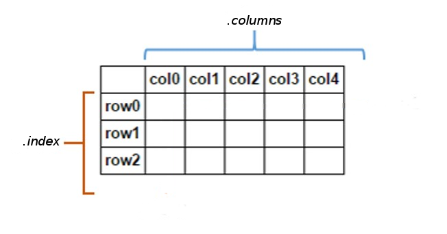Figure source: Reference [2].

The first column with the indices in pandas DataFrames does not need to be a sequence of integers, but it can also contain strings or other numeric data (e.g., dates, years).

For instance, let’s create a DataFrame called bacteria to see how indexing with string indices works. We again pass in a dictionary, with the keys corresponding to column names and the values to the data, and in addition we pass a list of strings called index. (Compare to the simple_table above, which does not use index for creating the DataFrame, and in that case, the indices were automatically set to integer numbers.)

bacteria = pd.DataFrame({'bacteria_counts' : [632, 1638, 569, 115],
                         'other_feature' : [438, 833, 234, 298]},
                         index=['Firmicutes', 'Proteobacteria', 'Actinobacteria', 'Bacteroidetes'])
bacteria

	bacteria_counts	other_feature
Firmicutes	632	438
Proteobacteria	1638	833
Actinobacteria	569	234
Bacteroidetes	115	298

To return the labels for the columns and indices of a DataFrame in pandas, we can use the methods shown in the following celss. Note again that the type of the returned objects is Index object.

bacteria.columns

Index(['bacteria_counts', 'other_feature'], dtype='object')

bacteria.index

Index(['Firmicutes', 'Proteobacteria', 'Actinobacteria', 'Bacteroidetes'], dtype='object')

For selecting rows and/or columns in pandas, beside the use of square brackets, two other operators are used: .loc and .iloc.

The operator .loc accesses rows by using string indices (i.e., string locations), that is, it uses the labels of the rows for indexing.

The operator .iloc accesses rows by using integer indices (i.e., integer locations), that is, it uses the integer positions of the rows for indexing.

The operators .loc and .iloc can accept either a single index (e.g., 'f' or 5), a list of indices (e.g., ['a','f'] or [2,5]), or a slice of indices (e.g., 'a:f' or 2:5).

For instance, if we are interested in accessing the row Actinobacteria, we can use .loc and the index name. This returns the column values for the specified row.

bacteria.loc['Actinobacteria']

bacteria_counts    569
other_feature      234
Name: Actinobacteria, dtype: int64

The operator .iloc does not work with string indices, and it returns an error in the following cell.

bacteria.iloc['Actinobacteria']

---------------------------------------------------------------------------
TypeError                                 Traceback (most recent call last)
Cell In[41], line 1
----> 1 bacteria.iloc['Actinobacteria']

File ~\AppData\Local\anaconda3\Lib\site-packages\pandas\core\indexing.py:1191, in _LocationIndexer.__getitem__(self, key)
   1189 maybe_callable = com.apply_if_callable(key, self.obj)
   1190 maybe_callable = self._check_deprecated_callable_usage(key, maybe_callable)
-> 1191 return self._getitem_axis(maybe_callable, axis=axis)

File ~\AppData\Local\anaconda3\Lib\site-packages\pandas\core\indexing.py:1749, in _iLocIndexer._getitem_axis(self, key, axis)
   1747 key = item_from_zerodim(key)
   1748 if not is_integer(key):
-> 1749     raise TypeError("Cannot index by location index with a non-integer key")
   1751 # validate the location
   1752 self._validate_integer(key, axis)

TypeError: Cannot index by location index with a non-integer key

To access rows with .iloc, we need to provide integer indices. Note that we can still access the row with iloc, even though the indices are strings.

bacteria.iloc[2]

bacteria_counts    569
other_feature      234
Name: Actinobacteria, dtype: int64

In addition, we can also use “positional indexing” with square brackets [], as in slicing operations with list and other sequence objects.

bacteria[2:3]

	bacteria_counts	other_feature
Actinobacteria	569	234

However, pandas doesn’t support indexing for accessing individual rows, and with positional indexing we need to use a slice (as in the above example bacteria[2:3]), otherwise, we will get an error.

bacteria[2]

---------------------------------------------------------------------------
KeyError                                  Traceback (most recent call last)
File ~\AppData\Local\anaconda3\Lib\site-packages\pandas\core\indexes\base.py:3805, in Index.get_loc(self, key)
   3804 try:
-> 3805     return self._engine.get_loc(casted_key)
   3806 except KeyError as err:

File index.pyx:167, in pandas._libs.index.IndexEngine.get_loc()

File index.pyx:196, in pandas._libs.index.IndexEngine.get_loc()

File pandas\\_libs\\hashtable_class_helper.pxi:7081, in pandas._libs.hashtable.PyObjectHashTable.get_item()

File pandas\\_libs\\hashtable_class_helper.pxi:7089, in pandas._libs.hashtable.PyObjectHashTable.get_item()

KeyError: 2

The above exception was the direct cause of the following exception:

KeyError                                  Traceback (most recent call last)
Cell In[44], line 1
----> 1 bacteria[2]

File ~\AppData\Local\anaconda3\Lib\site-packages\pandas\core\frame.py:4102, in DataFrame.__getitem__(self, key)
   4100 if self.columns.nlevels > 1:
   4101     return self._getitem_multilevel(key)
-> 4102 indexer = self.columns.get_loc(key)
   4103 if is_integer(indexer):
   4104     indexer = [indexer]

File ~\AppData\Local\anaconda3\Lib\site-packages\pandas\core\indexes\base.py:3812, in Index.get_loc(self, key)
   3807     if isinstance(casted_key, slice) or (
   3808         isinstance(casted_key, abc.Iterable)
   3809         and any(isinstance(x, slice) for x in casted_key)
   3810     ):
   3811         raise InvalidIndexError(key)
-> 3812     raise KeyError(key) from err
   3813 except TypeError:
   3814     # If we have a listlike key, _check_indexing_error will raise
   3815     #  InvalidIndexError. Otherwise we fall through and re-raise
   3816     #  the TypeError.
   3817     self._check_indexing_error(key)

KeyError: 2

There is another important difference between the above two selections, as .loc and .iloc return a Series object because we selected a single label, while [2:3] returns a DataFrame because we selected a range of positions. Let’s check this.

type(bacteria.loc['Actinobacteria'])

pandas.core.series.Series

type(bacteria.iloc[2])

pandas.core.series.Series

type(bacteria[2:3])

pandas.core.frame.DataFrame

Let’s return to the unemployment data to show how .iloc is used, since unemployment has integer indices.

unemployment.iloc[0:4]

	country	seasonality	year_month	unemployment	unemployment_rate
0	at	nsa	1993.01	171000	4.5
1	at	nsa	1993.02	175000	4.6
2	at	nsa	1993.03	166000	4.4
3	at	nsa	1993.04	157000	4.1

Note also that we can use loc with integer indices as well, however the output is different than .iloc. The difference is discussed in an upcoming section below.

unemployment.loc[0:4]

	country	seasonality	year_month	unemployment	unemployment_rate
0	at	nsa	1993.01	171000	4.5
1	at	nsa	1993.02	175000	4.6
2	at	nsa	1993.03	166000	4.4
3	at	nsa	1993.04	157000	4.1
4	at	nsa	1993.05	147000	3.9

Selecting a Specific Value

Both .loc and .iloc can be used to select a particular value if they are given two arguments. The first argument is the row name (when using .loc) or the row index number (when using .iloc), while the second argument is the column name or index number.

Using .loc, we can select “Bacteroidetes” and “bacteria_counts” to get the count of Bacteroidetes, as in the next cell below.

bacteria

	bacteria_counts	other_feature
Firmicutes	632	438
Proteobacteria	1638	833
Actinobacteria	569	234
Bacteroidetes	115	298

bacteria.loc['Bacteroidetes']['bacteria_counts']

np.int64(115)

# This is the same as above
bacteria.iloc[3][0]

C:\Users\vakanski\AppData\Local\Temp\ipykernel_21848\1562859839.py:2: FutureWarning: Series.__getitem__ treating keys as positions is deprecated. In a future version, integer keys will always be treated as labels (consistent with DataFrame behavior). To access a value by position, use `ser.iloc[pos]`
  bacteria.iloc[3][0]

np.int64(115)

# This the same as above
bacteria.iloc[3]['bacteria_counts']

np.int64(115)

Or, for the unemployment data:

# The year_month in the first row
unemployment.iloc[0,2]

np.float64(1993.01)

# This the same as above
unemployment.iloc[0][2]

C:\Users\vakanski\AppData\Local\Temp\ipykernel_21848\2135515946.py:2: FutureWarning: Series.__getitem__ treating keys as positions is deprecated. In a future version, integer keys will always be treated as labels (consistent with DataFrame behavior). To access a value by position, use `ser.iloc[pos]`
  unemployment.iloc[0][2]

np.float64(1993.01)

Selecting Multiple Rows and Columns

Both .loc and .iloc can be used to select subsets of rows and columns at the same time if they are given lists as arguments, or slices for .iloc.

The following example uses a list with .iloc to select specific rows, similar to fancy indexing in NumPy.

unemployment.iloc[[1, 5, 6, 22]]

	country	seasonality	year_month	unemployment	unemployment_rate
1	at	nsa	1993.02	175000	4.6
5	at	nsa	1993.06	134000	3.5
6	at	nsa	1993.07	128000	3.4
22	at	nsa	1994.11	148000	3.9

We can also select a range of rows and specify the step value.

unemployment.iloc[25:50:5]

	country	seasonality	year_month	unemployment	unemployment_rate
25	at	nsa	1995.02	174000	4.5
30	at	nsa	1995.07	123000	3.3
35	at	nsa	1995.12	175000	4.7
40	at	nsa	1996.05	159000	4.3
45	at	nsa	1996.10	146000	3.9

And we can apply slicing over rows and columns.

unemployment.iloc[2:6,0:2]

	country	seasonality
2	at	nsa
3	at	nsa
4	at	nsa
5	at	nsa

The following example selects multiple rows with .loc based on string indices.

bacteria.loc[['Firmicutes', 'Actinobacteria']]

	bacteria_counts	other_feature
Firmicutes	632	438
Actinobacteria	569	234

We can also select a subset of rows and columns with .loc.

bacteria.loc[['Bacteroidetes', 'Actinobacteria'], ['bacteria_counts']]

	bacteria_counts
Bacteroidetes	115
Actinobacteria	569

Using .iloc on the unemployment DataFrame, select the rows starting at row 2 and ending at row 5, and the 0th, 2nd, and 3rd columns.

unemployment.iloc[2:6,[0,2,3]]

	country	year_month	unemployment
2	at	1993.03	166000
3	at	1993.04	157000
4	at	1993.05	147000
5	at	1993.06	134000

The same selection can be achieved by using the .loc operator and listing the column names.

# The same as above
unemployment.loc[2:6,['country', 'year_month', 'unemployment']]

	country	year_month	unemployment
2	at	1993.03	166000
3	at	1993.04	157000
4	at	1993.05	147000
5	at	1993.06	134000
6	at	1993.07	128000

Selecting Multiple Rows and Columns Using Conditional Expressions

We can also display values from a DataFrame that satisfy certain criteria using conditional expressions, such as <, >, ==, !=, etc.

One example is shown below where only the rows that have an unemployment rate greater than 15 are shown.

unemployment[unemployment['unemployment_rate'] > 15].head(10)

	country	seasonality	year_month	unemployment	unemployment_rate
1717	bg	nsa	2000.02	523000	15.4
1718	bg	nsa	2000.03	547000	16.0
1719	bg	nsa	2000.04	560000	16.3
1720	bg	nsa	2000.05	561000	16.3
1721	bg	nsa	2000.06	554000	16.2
1722	bg	nsa	2000.07	558000	16.3
1723	bg	nsa	2000.08	569000	16.7
1724	bg	nsa	2000.09	574000	16.8
1725	bg	nsa	2000.10	583000	17.1
1726	bg	nsa	2000.11	597000	17.5

The following cells present one more example of selecting rows based on conditional statements.

score_df = pd.DataFrame(
    {'age': [17, 19, 21, 37, 18, 19, 47, 18, 19],
     'score': [12, 10, 11, 15, 16, 14, 25, 21, 29],
     'rt': [3.552, 1.624, 6.431, 7.132, 2.925, 4.662, 3.634, 3.635, 5.234],
     'group': ["test", "test", "test", "test", "test", "control", "control", "control", "control"]
    })

score_df

	age	score	rt	group
0	17	12	3.552	test
1	19	10	1.624	test
2	21	11	6.431	test
3	37	15	7.132	test
4	18	16	2.925	test
5	19	14	4.662	control
6	47	25	3.634	control
7	18	21	3.635	control
8	19	29	5.234	control

# select only rows from the 'test' group
df_test = score_df[score_df['group'] == 'test']
df_test

	age	score	rt	group
0	17	12	3.552	test
1	19	10	1.624	test
2	21	11	6.431	test
3	37	15	7.132	test
4	18	16	2.925	test

# select only rows for age > 19
df_adult = score_df[score_df['age']> 19]
df_adult

	age	score	rt	group
2	21	11	6.431	test
3	37	15	7.132	test
6	47	25	3.634	control

# select only rows for age > 19 and rt
adult_and_rt = score_df[(score_df['age'] > 19) & (score_df['rt'] > 3)]
adult_and_rt

	age	score	rt	group
2	21	11	6.431	test
3	37	15	7.132	test
6	47	25	3.634	control

# select only rows for age and rt in test group
adult_and_rt_test = score_df[(score_df['age'] > 19) & (score_df['rt'] > 3) & (score_df['group'] == 'test')]
adult_and_rt_test

	age	score	rt	group
2	21	11	6.431	test
3	37	15	7.132	test

Differences between loc and iloc

To show the differences between loc and iloc let’s consider the following example.

df1 = pd.DataFrame({'x':[10, 20, 30, 40 ,50],
                    'y':[20, 30, 40, 50, 60],
                    'z':[30, 40, 50, 60, 70]},
                      index=[10, 11,12, 0, 1])
df1

	x	y	z
10	10	20	30
11	20	30	40
12	30	40	50
0	40	50	60
1	50	60	70

Note in the following cells that df1.iloc[0] selects the row with index location 0, whereas loc selects the row with index label 0.

 # value at index location 0
df1.iloc[0]

x    10
y    20
z    30
Name: 10, dtype: int64

 # value at index label 0
df1.loc[0]

x    40
y    50
z    60
Name: 0, dtype: int64

Also, there is a difference in the selected rows when using slicing operations with iloc and loc. One must be careful when using these operators, and always check the output to ensure it is as expected.

# rows at index location between 0 and 1 (exclusive)
df1.iloc[0:1]

	x	y	z
10	10	20	30

# rows at index labels between 0 and 1 (inclusive)
df1.loc[0:1]

	x	y	z
0	40	50	60
1	50	60	70

7.4 Creating New Columns, Reordering

To create a new column in a DataFrame, we simply assign values to the new column, as in:

df['New_Column'] = ...

Often, the new columns are created from existing columns based on certain conditions, or by applying functions to existing columns.

Condition-Based: df['New_Column'] = df['Existing_Column'] > value
Function-Based: df['New_Column'] = df['Existing_Column'].apply(function)

Since the year_month column is not shown correctly in the unemployment DataFrame, let’s try to split it into two separate columns for years and months.

In the previous section, we saw that the data type in this column is float64. We will first extract the year using the .astype() method. This allows for type casting, i.e., using .astype(int) we will convert the floating point values into integer numbers (by truncating the decimals).

The new column year will be added on the right of the DataFrame.

unemployment['year'] = unemployment['year_month'].astype(int)
unemployment.head()

	country	seasonality	year_month	unemployment	unemployment_rate	year
0	at	nsa	1993.01	171000	4.5	1993
1	at	nsa	1993.02	175000	4.6	1993
2	at	nsa	1993.03	166000	4.4	1993
3	at	nsa	1993.04	157000	4.1	1993
4	at	nsa	1993.05	147000	3.9	1993

Next, let’s create a new column month. We will subtract the year value from year_month to get the decimal portion of the value, and multiply the result by 100 and convert to int. Because of the truncating that occurs when casting to int, we first need to round the values to the nearest whole number using round().

unemployment['month'] = ((unemployment['year_month'] - unemployment['year']) * 100).round().astype(int)
unemployment.head(12)

	country	seasonality	year_month	unemployment	unemployment_rate	year	month
0	at	nsa	1993.01	171000	4.5	1993	1
1	at	nsa	1993.02	175000	4.6	1993	2
2	at	nsa	1993.03	166000	4.4	1993	3
3	at	nsa	1993.04	157000	4.1	1993	4
4	at	nsa	1993.05	147000	3.9	1993	5
5	at	nsa	1993.06	134000	3.5	1993	6
6	at	nsa	1993.07	128000	3.4	1993	7
7	at	nsa	1993.08	130000	3.4	1993	8
8	at	nsa	1993.09	132000	3.5	1993	9
9	at	nsa	1993.10	141000	3.7	1993	10
10	at	nsa	1993.11	156000	4.1	1993	11
11	at	nsa	1993.12	169000	4.4	1993	12

Now, let’s try to reorder the newly created year and month columns in the DataFrame. For this, we will use the square brackets notation again, passing in a list of column names in the order we would like to see them.

unemployment = unemployment[['country', 'seasonality',
                             'year_month', 'year', 'month',
                             'unemployment', 'unemployment_rate']]
unemployment.head(10)

	country	seasonality	year_month	year	month	unemployment	unemployment_rate
0	at	nsa	1993.01	1993	1	171000	4.5
1	at	nsa	1993.02	1993	2	175000	4.6
2	at	nsa	1993.03	1993	3	166000	4.4
3	at	nsa	1993.04	1993	4	157000	4.1
4	at	nsa	1993.05	1993	5	147000	3.9
5	at	nsa	1993.06	1993	6	134000	3.5
6	at	nsa	1993.07	1993	7	128000	3.4
7	at	nsa	1993.08	1993	8	130000	3.4
8	at	nsa	1993.09	1993	9	132000	3.5
9	at	nsa	1993.10	1993	10	141000	3.7

Here is one more example of creating new columns by applying functions to existing columns.

student_df = pd.DataFrame({
    'Student': ['Alice', 'Bob', 'Charlie', 'David', 'Eve'],
    'Score': [85, 80, 78, 92, 68]})
student_df

	Student	Score
0	Alice	85
1	Bob	80
2	Charlie	78
3	David	92
4	Eve	68

# add 10 marks
student_df['Updated Score'] = student_df['Score'] + 10
student_df

	Student	Score	Updated Score
0	Alice	85	95
1	Bob	80	90
2	Charlie	78	88
3	David	92	102
4	Eve	68	78

# esnure scores are not greater than 100
student_df['Final Score'] = student_df['Updated Score'].clip(upper=100)
student_df

	Student	Score	Updated Score	Final Score
0	Alice	85	95	95
1	Bob	80	90	90
2	Charlie	78	88	88
3	David	92	102	100
4	Eve	68	78	78

# calculate mean and standard deviation (rounded to 2 decimal places)
student_df['Mean Score'] = student_df['Score'].mean()
student_df['Standard Deviation'] = round(student_df['Final Score'].std(),2)
student_df

	Student	Score	Updated Score	Final Score	Mean Score	Standard Deviation
0	Alice	85	95	95	80.6	8.26
1	Bob	80	90	90	80.6	8.26
2	Charlie	78	88	88	80.6	8.26
3	David	92	102	100	80.6	8.26
4	Eve	68	78	78	80.6	8.26

7.5 Removing Columns and Rows

To delete a column from a DataFrame, we can use the the drop() method. For instance, in the countries DataFrame, we will drop the column country_group. With the drop() method it is important to specify the axis parameter, where axis=1 refers to columns (axis=0 refers to rows).

countries.head()

	country	google_country_code	country_group	name_en	name_fr	name_de	latitude	longitude
0	at	AT	eu	Austria	Autriche	Österreich	47.696554	13.345980
1	be	BE	eu	Belgium	Belgique	Belgien	50.501045	4.476674
2	bg	BG	eu	Bulgaria	Bulgarie	Bulgarien	42.725674	25.482322
3	hr	HR	non-eu	Croatia	Croatie	Kroatien	44.746643	15.340844
4	cy	CY	eu	Cyprus	Chypre	Zypern	35.129141	33.428682

countries.drop('country_group', axis=1, inplace=True)
countries.head()

	country	google_country_code	name_en	name_fr	name_de	latitude	longitude
0	at	AT	Austria	Autriche	Österreich	47.696554	13.345980
1	be	BE	Belgium	Belgique	Belgien	50.501045	4.476674
2	bg	BG	Bulgaria	Bulgarie	Bulgarien	42.725674	25.482322
3	hr	HR	Croatia	Croatie	Kroatien	44.746643	15.340844
4	cy	CY	Cyprus	Chypre	Zypern	35.129141	33.428682

By using the drop() method we can remove multiple columns, by listing their labels within a list.

countries.drop(['latitude', 'longitude'], axis=1, inplace=True)
countries.head()

	country	google_country_code	name_en	name_fr	name_de
0	at	AT	Austria	Autriche	Österreich
1	be	BE	Belgium	Belgique	Belgien
2	bg	BG	Bulgaria	Bulgarie	Bulgarien
3	hr	HR	Croatia	Croatie	Kroatien
4	cy	CY	Cyprus	Chypre	Zypern

Another way to remove columns in pandas is by using the del keyword.

del countries['google_country_code']
countries.head()

	country	name_en	name_fr	name_de
0	at	Austria	Autriche	Österreich
1	be	Belgium	Belgique	Belgien
2	bg	Bulgaria	Bulgarie	Bulgarien
3	hr	Croatia	Croatie	Kroatien
4	cy	Cyprus	Chypre	Zypern

To remove rows from a DataFrame, we can use the drop() method and set the axis parameter to 0.

Similarly to columns, we can delete a single row, or multiple rows as in the examples below.

unemployment.drop(3, axis=0, inplace=True)
unemployment.head()

	country	seasonality	year_month	year	month	unemployment	unemployment_rate
0	at	nsa	1993.01	1993	1	171000	4.5
1	at	nsa	1993.02	1993	2	175000	4.6
2	at	nsa	1993.03	1993	3	166000	4.4
4	at	nsa	1993.05	1993	5	147000	3.9
5	at	nsa	1993.06	1993	6	134000	3.5

unemployment.drop([6,8], axis=0, inplace=True)
unemployment.head(10)

	country	seasonality	year_month	year	month	unemployment	unemployment_rate
0	at	nsa	1993.01	1993	1	171000	4.5
1	at	nsa	1993.02	1993	2	175000	4.6
2	at	nsa	1993.03	1993	3	166000	4.4
4	at	nsa	1993.05	1993	5	147000	3.9
5	at	nsa	1993.06	1993	6	134000	3.5
7	at	nsa	1993.08	1993	8	130000	3.4
9	at	nsa	1993.10	1993	10	141000	3.7
10	at	nsa	1993.11	1993	11	156000	4.1
11	at	nsa	1993.12	1993	12	169000	4.4
12	at	nsa	1994.01	1994	1	180000	4.7

# Check the shape of the modified DataFrame
unemployment.shape

(20793, 7)

Another common way to remove columns or rows is based on a certain condition. For example, the following condition removes all rows corresponding to the data after 2006.

unemployment = unemployment[unemployment['year'] < 2006]

# Check the shape again
unemployment.shape

(15528, 7)

7.6 Merging DataFrames

Merging DataFrames in pandas is a common operation for combining data from multiple DataFrames based on a common key or index.

For instance, if we examine the unemployment DataFrame we can notice that we don’t exactly know what the values in the country column refer to. We can correct that by obtaining the country names from the countries DataFrame that we imported earlier.

We can see in the countries data that at stands for Austria. This DataFrame even provides the country names in three different languages (name_en, name_fr, name_de).

countries.head()

	country	name_en	name_fr	name_de
0	at	Austria	Autriche	Österreich
1	be	Belgium	Belgique	Belgien
2	bg	Bulgaria	Bulgarie	Bulgarien
3	hr	Croatia	Croatie	Kroatien
4	cy	Cyprus	Chypre	Zypern

Because the data we need is stored in two separate files, we will merge the two DataFrames. The country column is shown in both DataFrames, so it is a good option for joining the data. However, we don’t need all columns in the countries DataFrame, and therefore, we will create a new DataFrame that contains only the columns that we need. To select certain columns to retain, we can use the bracket notation that we used earlier to reorder the columns.

country_names = countries[['country', 'name_en']]

country_names.head(5)

	country	name_en
0	at	Austria
1	be	Belgium
2	bg	Bulgaria
3	hr	Croatia
4	cy	Cyprus

For merging DataFrames, pandas include the merge method, which has the following syntax, where the parameter on lists the column for matching the DataFrames. This operation is similar to inner join in SQL and it combines rows which have matching keys in both DataFrames. We can also specify the type of join (e.g., inner, left, right, outer) by providing value for the optional how parameter.

pd.merge(first_file, second_file, on=['column_name'], how=['join type (default is 'inner')])

unemployment = pd.merge(unemployment, country_names, on=['country'])
unemployment.head()

	country	seasonality	year_month	year	month	unemployment	unemployment_rate	name_en
0	at	nsa	1993.01	1993	1	171000	4.5	Austria
1	at	nsa	1993.02	1993	2	175000	4.6	Austria
2	at	nsa	1993.03	1993	3	166000	4.4	Austria
3	at	nsa	1993.05	1993	5	147000	3.9	Austria
4	at	nsa	1993.06	1993	6	134000	3.5	Austria

If we want to merge two files using multiple columns that exist in both files, we can pass a list of column names to the on parameter.

Combining DataFrames with join() and concat()

Another similar method to merge that is used for combining DataFrames in pandas is join(). The join() function is often used for merging DataFrame based on index alignment.

The following example joins the DataFrame grades_df to the student_df by matching the index positions between the DataFrames. This is equivalent to a left join operation.

student_df = pd.DataFrame({
    'Student': ['Alice', 'Bob', 'Charlie', 'David', 'Eve'],
    'Score': [85, 80, 78, 92, 68]})
student_df

	Student	Score
0	Alice	85
1	Bob	80
2	Charlie	78
3	David	92
4	Eve	68

grades_df = pd.DataFrame({'Grade': ['A', 'B', 'A', 'C']}, index=[1, 2, 3, 4])
grades_df

	Grade
1	A
2	B
3	A
4	C

joined_df = student_df.join(grades_df)
joined_df

	Student	Score	Grade
0	Alice	85	NaN
1	Bob	80	A
2	Charlie	78	B
3	David	92	A
4	Eve	68	C

However, join() also allows to specify the type of join operation with the how argument, similar to merge(). In the example below, an inner join operation is illustrated, which returns the rows that have matching indices in both DataFrames.

joined_df = student_df.join(grades_df, how='inner')
joined_df

	Student	Score	Grade
1	Bob	80	A
2	Charlie	78	B
3	David	92	A
4	Eve	68	C

Note again the join() is primarily designed for merging DataFrames based on their indices, and it does not support merging DatFrames on specific columns. For that purpose, we should use the merge() method instead.

Similarly, concat() allows to combine two DataFrames in pandas along a particular axis (either rows or columns). By default, it includes all columns or rows, filling missing values with NaN. However, the concat function can also accept a join argument to specify the type of join operation.

# Concatenate along columns (axis=1)
joined_df_2 = pd.concat([student_df, grades_df], axis=1)
joined_df_2

	Student	Score	Grade
0	Alice	85	NaN
1	Bob	80	A
2	Charlie	78	B
3	David	92	A
4	Eve	68	C

# Concatenate along rows (axis=0)
student_df_2 = pd.DataFrame({'Student': ['George', 'Ann'], 'Score': [69, 82]})
joined_df_3 = pd.concat([student_df, student_df_2], axis=0)
joined_df_3

	Student	Score
0	Alice	85
1	Bob	80
2	Charlie	78
3	David	92
4	Eve	68
0	George	69
1	Ann	82

In the combined DataFrame joined_df_3 above, notice that the indices of the added rows begin at 0. To reset the indices in a pandas DataFrame, we can use, well, the reset_index() method.

joined_df_3 = joined_df_3.reset_index()
joined_df_3

	index	Student	Score
0	0	Alice	85
1	1	Bob	80
2	2	Charlie	78
3	3	David	92
4	4	Eve	68
5	0	George	69
6	1	Ann	82

For more information on merging DataFrames, check the pandas documentation. Also, we will explain more about merging operations in the lecture on Databases and SQL.

Here is a figure that depicts inner, right, left, and outer join operations.

Figure: Join Operations.

7.7 Calculating Unique and Missing Values

In the unemployment DataFrame, we might want to know for which countries we have data available. To extract this information, we can use the .unique() method. Note that the countries are listed in the right-most column name-en so we will use it to find the unique elements in that column.

unemployment.head()

	country	seasonality	year_month	year	month	unemployment	unemployment_rate	name_en
0	at	nsa	1993.01	1993	1	171000	4.5	Austria
1	at	nsa	1993.02	1993	2	175000	4.6	Austria
2	at	nsa	1993.03	1993	3	166000	4.4	Austria
3	at	nsa	1993.05	1993	5	147000	3.9	Austria
4	at	nsa	1993.06	1993	6	134000	3.5	Austria

unemployment['name_en'].unique()

array(['Austria', 'Belgium', 'Bulgaria', 'Cyprus', 'Czech Republic',
       'Germany (including  former GDR from 1991)', 'Denmark', 'Estonia',
       'Spain', 'Finland', 'France', 'Greece', 'Croatia', 'Hungary',
       'Ireland', 'Italy', 'Lithuania', 'Luxembourg', 'Latvia', 'Malta',
       'Netherlands', 'Norway', 'Poland', 'Portugal', 'Romania', 'Sweden',
       'Slovenia', 'Slovakia', 'Turkey', 'United Kingdom'], dtype=object)

To get a count of the number of unique countries, we can use the .nunique() method.

unemployment['name_en'].nunique()

30

Or, we can also use len() to get the number of items in the above array.

len(unemployment['name_en'].unique())

30

If we are interested to know how many rows there are per country, pandas has the .value_counts() method that returns the counts for the unique values in a column.

unemployment['name_en'].value_counts()

name_en
Belgium                                      828
Denmark                                      828
Spain                                        828
France                                       828
Luxembourg                                   828
Ireland                                      828
Portugal                                     828
Netherlands                                  828
United Kingdom                               828
Sweden                                       828
Italy                                        804
Finland                                      648
Norway                                       612
Austria                                      465
Slovakia                                     396
Slovenia                                     396
Malta                                        396
Poland                                       396
Bulgaria                                     396
Hungary                                      396
Germany (including  former GDR from 1991)    336
Czech Republic                               288
Latvia                                       288
Lithuania                                    288
Greece                                       279
Romania                                      252
Cyprus                                       216
Estonia                                      216
Croatia                                      144
Turkey                                        36
Name: count, dtype: int64

By default, the output is sorted by values in descending order. If we would like it sorted by index (or, by country name in alphabetical order in this case), we can append the .sort_index() method.

unemployment['name_en'].value_counts().sort_index()

name_en
Austria                                      465
Belgium                                      828
Bulgaria                                     396
Croatia                                      144
Cyprus                                       216
Czech Republic                               288
Denmark                                      828
Estonia                                      216
Finland                                      648
France                                       828
Germany (including  former GDR from 1991)    336
Greece                                       279
Hungary                                      396
Ireland                                      828
Italy                                        804
Latvia                                       288
Lithuania                                    288
Luxembourg                                   828
Malta                                        396
Netherlands                                  828
Norway                                       612
Poland                                       396
Portugal                                     828
Romania                                      252
Slovakia                                     396
Slovenia                                     396
Spain                                        828
Sweden                                       828
Turkey                                        36
United Kingdom                               828
Name: count, dtype: int64

As we noticed earlier, there are missing values in the unemployment_rate column. To find out how many unemployment rate values are missing we will use the .isnull() method, which returns a corresponding boolean value for each missing entry in the unemployment_rate column. As we know, in Python True is equivalent to 1 and False is equivalent to 0. Thus, when we add .sum(), we obtain a count for the total number of missing values in the unemployment_rate column.

unemployment['unemployment_rate'].isnull().sum()

np.int64(825)

GroupBy

The groupby() method in pandas is used to group data based on one or more columns. It is similar to the GroupBy function in SQL, and allows to apply operations or filtering on grouped data.

The general syntax is shown below, meaning split the data in another_column into groups based on the column_name and use an aggregation function (like sum, min, max, etc.) to combine the results.

df.groupby('column_name')['another_column'].aggregation_function()

If we would like to know how many missing values for the unemployment_rate column there are for each country, we can first create a new column in the DataFrame that has boolean True or False for the unemployment_rate column. This is the last column to the right below, in which False means that the value is not missing.

unemployment['unemployment_rate_null'] = unemployment['unemployment_rate'].isnull()
unemployment.head()

	country	seasonality	year_month	year	month	unemployment	unemployment_rate	name_en	unemployment_rate_null
0	at	nsa	1993.01	1993	1	171000	4.5	Austria	False
1	at	nsa	1993.02	1993	2	175000	4.6	Austria	False
2	at	nsa	1993.03	1993	3	166000	4.4	Austria	False
3	at	nsa	1993.05	1993	5	147000	3.9	Austria	False
4	at	nsa	1993.06	1993	6	134000	3.5	Austria	False

To count the number of missing values for each country, we can use the .groupby() method to group the data by the country name_en column included in the parentheses, and perform the .sum() operation over the unemployment_rate_null column.

unemployment.groupby('name_en')['unemployment_rate_null'].sum()

name_en
Austria                                        0
Belgium                                        0
Bulgaria                                     180
Croatia                                       96
Cyprus                                         0
Czech Republic                                 0
Denmark                                        0
Estonia                                        0
Finland                                        0
France                                         0
Germany (including  former GDR from 1991)      0
Greece                                         0
Hungary                                       36
Ireland                                        0
Italy                                          0
Latvia                                         0
Lithuania                                      0
Luxembourg                                     0
Malta                                        180
Netherlands                                    0
Norway                                         0
Poland                                        72
Portugal                                       0
Romania                                        0
Slovakia                                     108
Slovenia                                      36
Spain                                        117
Sweden                                         0
Turkey                                         0
United Kingdom                                 0
Name: unemployment_rate_null, dtype: int64

Also, we can use .groupby to group data by multiple columns, as in

df.groupby(['column_name1', 'column_name2'])['another_column'].aggregation_function()

For example, we can check the missing values for unemployment both by country and year, and we can apply functions such as .sum() to the grouped objects, as shown below.

grouped_sum = unemployment.groupby(['name_en', 'year'])['unemployment_rate_null'].sum()

# Convert to a DataFrame
grouped_sum_df = grouped_sum.to_frame()
grouped_sum_df

		unemployment_rate_null
name_en	year
Austria	1993	0
	1994	0
	1995	0
	1996	0
	1997	0
...	...	...
United Kingdom	2001	0
	2002	0
	2003	0
	2004	0
	2005	0

437 rows × 1 columns

One more simple example of using groupby in pandas is shown below.

company_df = pd.DataFrame({
    'Department': ['HR', 'IT', 'HR', 'IT', 'IT', 'HR'],
    'Employee': ['Alice', 'Bob', 'Charlie', 'David', 'Edward', 'Fiona'],
    'Salary': [70000, 80000, 75000, 85000, 90000, 71000],
    'JobTitle' : ['Employee', 'Developer', 'Manager', 'Developer', 'Manager', 'Employee']
})

company_df

	Department	Employee	Salary	JobTitle
0	HR	Alice	70000	Employee
1	IT	Bob	80000	Developer
2	HR	Charlie	75000	Manager
3	IT	David	85000	Developer
4	IT	Edward	90000	Manager
5	HR	Fiona	71000	Employee

Group by the column 'Department and calculate the mean salary for each department.

company_df.groupby('Department')['Salary'].mean()

Department
HR    72000.0
IT    85000.0
Name: Salary, dtype: float64

We can perform multiple operations on the grouped data. The following example calculates the mean, sum, max, and min for the grouped data. These operations for calculating data statistics in pandas are referred to as aggregate functions. They are listed inside the agg() method, allowing to apply multiple operations at once.

company_df.groupby('Department').agg({
    'Salary': ['mean', 'sum', 'max', 'min']})

	Salary
	mean	sum	max	min
Department
HR	72000.0	216000	75000	70000
IT	85000.0	255000	90000	80000

We can group the data by 'Department' and 'JobTitle' and calculate the mean salary.

company_df.groupby(['Department', 'JobTitle'])['Salary'].mean()

Department  JobTitle
HR          Employee     70500.0
            Manager      75000.0
IT          Developer    82500.0
            Manager      90000.0
Name: Salary, dtype: float64

7.8 Dealing With Missing Values: Boolean Indexing

Two main options for dealing with missing values in a DataFrame include:

• Fill the missing values with some other values.

• Remove the observations with missing values.

Here we will adopt the second approach and exclude missing values from our primary analyses. Additional examples on dealing with missing values will be presented in the lecture on Data Exploration and Preprocessing.

To select only the rows with the missing data for 'unemployment_rate', we will use boolean indexing to filter the data. Recall from the previous section that unemployment['unemployment_rate'].isnull() produces an array of Boolean values, which we used when counting the number of missing values, shown in the next cell.

unemployment['unemployment_rate'].isnull()[:10]

0    False
1    False
2    False
3    False
4    False
5    False
6    False
7    False
8    False
9    False
Name: unemployment_rate, dtype: bool

We will first save the missing data into a new DataFrame, in case we need that data later. To create a new DataFrame that we will call unemployment_rate_missing, we will index unemployment with the Boolean array above. This returns only the rows where the value in the array is True.

unemployment_rate_missing = unemployment[unemployment['unemployment_rate'].isnull()]
unemployment_rate_missing.head()

	country	seasonality	year_month	year	month	unemployment	unemployment_rate	name_en	unemployment_rate_null
1293	bg	nsa	1995.01	1995	1	391000	NaN	Bulgaria	True
1294	bg	nsa	1995.02	1995	2	387000	NaN	Bulgaria	True
1295	bg	nsa	1995.03	1995	3	378000	NaN	Bulgaria	True
1296	bg	nsa	1995.04	1995	4	365000	NaN	Bulgaria	True
1297	bg	nsa	1995.05	1995	5	346000	NaN	Bulgaria	True

It is also possible to specify multiple conditions using the & operator, but each condition needs to be inside of parentheses.

Now, to remove the missing data in unemployment, we can use the .dropna() method. This method drops all observations for which unemployment_rate == NaN.

unemployment.dropna(subset=['unemployment_rate'], inplace=True)
unemployment.head()

	country	seasonality	year_month	year	month	unemployment	unemployment_rate	name_en	unemployment_rate_null
0	at	nsa	1993.01	1993	1	171000	4.5	Austria	False
1	at	nsa	1993.02	1993	2	175000	4.6	Austria	False
2	at	nsa	1993.03	1993	3	166000	4.4	Austria	False
3	at	nsa	1993.05	1993	5	147000	3.9	Austria	False
4	at	nsa	1993.06	1993	6	134000	3.5	Austria	False

# Check the shape of the modified DataFrame
unemployment.shape

(14703, 9)

Sorting Values

If we want to know what the highest unemployment rates were, we can use the .sort_values() method to sort the data.

The code in the next cell sorted the data in descending order, and printed the first 10 rows.

unemployment.sort_values('unemployment_rate', ascending=False)[:10]

	country	seasonality	year_month	year	month	unemployment	unemployment_rate	name_en	unemployment_rate_null
11677	pl	nsa	2004.02	2004	2	3531000	20.9	Poland	False
11676	pl	nsa	2004.01	2004	1	3520000	20.7	Poland	False
11665	pl	nsa	2003.02	2003	2	3460000	20.7	Poland	False
11664	pl	nsa	2003.01	2003	1	3466000	20.6	Poland	False
11678	pl	nsa	2004.03	2004	3	3475000	20.6	Poland	False
11654	pl	nsa	2002.03	2002	3	3509000	20.5	Poland	False
11666	pl	nsa	2003.03	2003	3	3417000	20.4	Poland	False
11653	pl	nsa	2002.02	2002	2	3492000	20.4	Poland	False
11925	pl	trend	2002.10	2002	10	3483000	20.4	Poland	False
11924	pl	trend	2002.09	2002	9	3500000	20.4	Poland	False

Here is another example for sorting the score_df DataFrame by 'age'.

score_df

	age	score	rt	group
0	17	12	3.552	test
1	19	10	1.624	test
2	21	11	6.431	test
3	37	15	7.132	test
4	18	16	2.925	test
5	19	14	4.662	control
6	47	25	3.634	control
7	18	21	3.635	control
8	19	29	5.234	control

score_df.sort_values('age')

	age	score	rt	group
0	17	12	3.552	test
4	18	16	2.925	test
7	18	21	3.635	control
1	19	10	1.624	test
5	19	14	4.662	control
8	19	29	5.234	control
2	21	11	6.431	test
3	37	15	7.132	test
6	47	25	3.634	control

The syntax shown in the next cell can also be used.

score_df.sort_values(by=['score'])

	age	score	rt	group
1	19	10	1.624	test
2	21	11	6.431	test
0	17	12	3.552	test
5	19	14	4.662	control
3	37	15	7.132	test
4	18	16	2.925	test
7	18	21	3.635	control
6	47	25	3.634	control
8	19	29	5.234	control

In the following code, we sort the data by two columns. Note that the data is first sorted by 'age', and for the rows where the age is the same (e.g., 18 or 19), the data is sorted in ascending order based on 'score'.

score_df.sort_values(['age', 'score'])

	age	score	rt	group
0	17	12	3.552	test
4	18	16	2.925	test
7	18	21	3.635	control
1	19	10	1.624	test
5	19	14	4.662	control
8	19	29	5.234	control
2	21	11	6.431	test
3	37	15	7.132	test
6	47	25	3.634	control

Several additional functionalities of pandas will be described in the next lectures.

7.9 Exporting A DataFrame to csv

To save the last DataFrame as a .csv file, we can use the .to_csv() method.

unemployment.to_csv('data/unemployment.csv')

The file will be saved in the data directory.

By default, this method writes the indices in the column 0 (i.e., row labels). We probably don’t want a column 0 with indices to be added, and we can set index to False. We can also specify the type of delimiter that we want to use, such as commas (,), pipes (|), semicolons (;), tabs (\t), etc.

unemployment.to_csv('data/unemployment.csv', index=False, sep=',')

References

1. Introduction to Pandas, Python Data Wrangling by D-Lab at UC Berkley, available at: https://github.com/dlab-berkeley/introduction-to-pandas.

2. Pandas documentation, available at: https://pandas.pydata.org/pandas-docs/stable/.

3. Learning Statistics with Python - Data Wrangling, available at: https://ethanweed.github.io/pythonbook/03.03-pragmatic_matters.html.

BACK TO TOP