Lecture 18 - Natural Language Processing¶

18.1 Introduction to NLP
18.2 Preprocessing Text Data
18.3 Text Tokenization
18.4 Representation of Groups of Words
18.5 Sequence Models Approach
References

18.1 Introduction to NLP¶

Natural Language Processing (NLP) is a branch of Computer Science (and more broadly, a branch of Artificial Intelligence) that is concerned with providing computers with the ability to understand texts and human language.

Common tasks in NLP include:

Text classification — assign a class label to text based on the topic discussed in the text, e.g., sentiment analysis (positive or negative movie review), spam detection, content filtering (detect abusive content).
Text summarization/reading comprehension — summarize a long input document with a shorter text.
Speech recognition — convert spoken language to text.
Machine translation — convert text in a source language to a target language.
Part of Speech (PoS) tagging — mark up words in text as nouns, verbs, adverbs, etc.
Question answering — output an answer to an input question.
Dialog generation — generate the next reply in a conversation given the history of the conversation.
Text generation — generate text to complete the sentence or to complete the paragraph.

18.2 Preprocessing Text Data¶

Before text data can be processed by NLP models, it must first be converted into a numerical representation.

Converting text into numerical form typically involves the following steps:

Standardization - remove punctuation, convert the text to lowercase.
Tokenization - break the text into smaller units called tokens (e.g., individual words, several consecutive words (N-grams), or individual characters).
Indexing - assign a unique numerical index to each token in the training set (i.e., build a vocabulary).
Embedding - (used in more recent models) assign a numerical vector to each token that represents it in a continuous vector space. Examples include one-hot encoding and word embeddings (explained in Section 18.5).

Note that differently from conventional NLP models that employ the text preprocessing steps listed above, Large Language Models (LLMs) typically apply minimal text processing and standardization, such as removing irregular spacing in text, removing non-textual content (e.g., code, HTML tags), and removing toxic or low-quality text content. Therefore, text preprocessing for LLM training focuses mainly on data cleanliness, and not on linguistic simplification. LLMs learn language structure directly from text data, and hence, it is preferred to keep all contextual information available for model training.

Text Standardization¶

Text standardization usually includes several steps, which depend on the specific application. The steps involve:

Remove punctuation marks (such as comma, period) or non-alphabetic characters (@, #, {, ]).
Change all words to lower-case letters, since ML models should consider Text and text as the same word.

Some NLP tasks apply additional steps, such as:

Correct spelling errors, or replace abbreviations with full words.
Remove stop words, such as for, the, is, to, some, etc.; if the task is text classification, these words are not relevant to the meaning of the text.
Apply stemming and lemmatization, which transform words to their base form, such as changing the word driving to drive, or grilled to grill since they have a common root.

Applying text standardization is helpful for training ML models, for example, because the models do not need to consider Text and text as two different words, which reduces the requirements for large training datasets. However, depending on the application, text standardization may remove information that can be important for some tasks, and this should always be considered when performing text preprocessing.

Tokenization¶

Tokenization is breaking up a sequence of text into individual units called tokens.

Tokenization can be performed at different levels:

Character-level tokenization - the text is divided into individual characters, and each character is a token, including letters, digits, punctuation marks, and symbols. One disadvantage of this type of tokenization is that anagrams (words with same letters in different order, such as silent and listen) can have the same numerical encoding, which can affect the performance of ML models. As well as, character-level tokenization does not capture semantic meaning of words as effectively as word-level tokens. Consequently, it is not widely used in practice.
Word-level tokenization - each word in the text is a token. This type of tokenization provides a natural representation of input text with the words as building blocks of language, and it is commonly used.
Subword-level tokenization - the words are divided into smaller units (e.g., tokenizing the word “unhappiness” into two tokens “un” + “happiness”). This type of tokenization is very common in recent Large Language Models. Also, in some languages with complex word structures, subword-level tokenization is the most suitable.
N-gram tokenization - N consecutive words represent a token. For instance, N-grams consisting of two adjacent words are called bigrams, or three words constitute a trigram, etc. N-gram tokens preserve the word order and can potentially capture more information in the text. For instance, for spam filtering using bigram tokens such as mailing list or bank account may provide more helpful information than using word-level tokens.

For some NLP tasks, tokenization can also be performed at other levels of text. An example is sentence-level tokenization for the task of document segmentation in sentences.

An example of text standardization, word-level tokenization, and indexing is shown in the next figure.

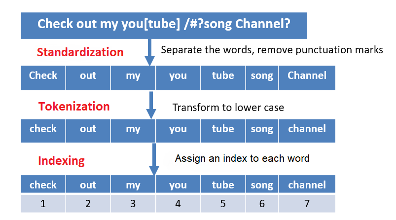
51cbfe0cdedf471ca00544de1f90a15f

Figure: Text standardization, word-level tokenization, and indexing.

18.3 Text Tokenization¶

TensorFlow-Keras library provides a text preprocessing function Tokenizer for converting raw text into sequences of tokens. The Tokenizer function performs text standardization, tokenization, and indexing.

The TensorFlow-Keras Tokenizer has the following arguments:

num_words: the maximum number of words to keep in the input text. It is recommended to set a high number if we are not sure what is the maximum number of words in the training set, because if we set a number less than the words in the text, some words will not be tokenized.
filters: by default, all punctuation and special characters in the text will be removed. If we want to change that, we can provide a list of punctuation and characters to keep.
lower: can be True or False. By default, it is True, and that means all texts will be converted to lowercase.
split: separator for splitting words. A default separator is a space (" ").
char_level: can be True or False. By default, it is False and will perform word-level tokenization. If it is True, the function will perform character-level tokenization.
oov_token: oov stands for Out Of Vocabulary, and it denotes a special token that will replace tokens that are not present in the input text.

18.3.1 Character-level Tokens¶

To use Tokenizer for character-level tokenization, we need to set char_level to True. Let’s set the number of tokens to 1,000.

Let’s apply it to the following sentence by using the method fit_on_texts().

[ ]:

import tensorflow as tf
import numpy as np

# Print the version of tf
print("TensorFlow version:{}".format(tf.__version__))

TensorFlow version:2.19.0

[ ]:

# A sample sentence
sentence = ['TensorFlow is a Machine Learning framework']

[ ]:

from tensorflow.keras.preprocessing.text import Tokenizer

character_tokenizer = Tokenizer(num_words=1000, char_level=True)

# Fitting tokenizer on sentences
character_tokenizer.fit_on_texts(sentence)

When the Tokenizer separates the characters in text, it creates a dictionary that maps each character to an integer index. We can inspect the dictionary by using the attribute word_index, although since we have set char_level to True in this case it is the character index.

Note that the start index is 1. By default, all letters are converted to lowercase. The first token is an empty space " ", the second is the letter 'e', etc. There are 17 unique characters in the sentence, including the empty space.

[ ]:

char_index = character_tokenizer.word_index
print(char_index)

{' ': 1, 'e': 2, 'n': 3, 'r': 4, 'a': 5, 'o': 6, 'i': 7, 's': 8, 'f': 9, 'l': 10, 'w': 11, 'm': 12, 't': 13, 'c': 14, 'h': 15, 'g': 16, 'k': 17}

The method text_to_sequences outputs the indices for the text. You can check that the word TensorFlow has the indices 13, 2, 3, 8, 6, 4, 9, 10, 6, 11, where each index corresponds to the letters listed in char_index.

[ ]:

print(character_tokenizer.texts_to_sequences(sentence))

[[13, 2, 3, 8, 6, 4, 9, 10, 6, 11, 1, 7, 8, 1, 5, 1, 12, 5, 14, 15, 7, 3, 2, 1, 10, 2, 5, 4, 3, 7, 3, 16, 1, 9, 4, 5, 12, 2, 11, 6, 4, 17]]

As we mentioned earlier, character-level tokenization is rarely used, because it does not capture semantic meaning of words as effectively as word-level tokens.

18.3.2 Word-level Tokens¶

To use the Tokenizer function for tokenizing words instead of characters, we need to just change the argument char_level to False, which is the default setting, so we may as well just omit it.

[ ]:

# Sample sentences
sentences = ['TensorFlow is a Machine Learning framework.',
             'Keras is a well designed deep learning API!',
             'Keras is built on top of TensorFlow!']

After the text is broken down into individual words, the Tokenizer builds a vocabulary of all words that are found in the input text, and assigns a unique integer index to each word in the vocabulary. We can inspect the words by using again the attribute word_index.

[ ]:

word_tokenizer = Tokenizer(num_words=1000)

# Fitting tokenizer on sentences
word_tokenizer.fit_on_texts(sentences)

word_index = word_tokenizer.word_index
print(word_index)

{'is': 1, 'tensorflow': 2, 'a': 3, 'learning': 4, 'keras': 5, 'machine': 6, 'framework': 7, 'well': 8, 'designed': 9, 'deep': 10, 'api': 11, 'built': 12, 'on': 13, 'top': 14, 'of': 15}

There are 15 unique words in the above sentences. By default, all punctuation are removed and all letters are converted to lowercase.

The indices for the above three sentences are shown below. For instance, the first list [2, 1, 3, 6, 4, 7] represents the first sentence in the text TensorFlow is a Machine Learning framework.

[ ]:

print(word_tokenizer.texts_to_sequences(sentences))

[[2, 1, 3, 6, 4, 7], [5, 1, 3, 8, 9, 10, 4, 11], [5, 1, 12, 13, 14, 15, 2]]

Also, word_counts can return the number of times each word appears in the sentences.

[ ]:

word_counts = word_tokenizer.word_counts
word_counts

OrderedDict([('tensorflow', 2),
             ('is', 3),
             ('a', 2),
             ('machine', 1),
             ('learning', 2),
             ('framework', 1),
             ('keras', 2),
             ('well', 1),
             ('designed', 1),
             ('deep', 1),
             ('api', 1),
             ('built', 1),
             ('on', 1),
             ('top', 1),
             ('of', 1)])

Out of Vocabulary Words¶

To handle the case when the Tokenizer is applied to text that contains words that were not present in the original documents, we can define a special token called oov_token. This token will be used to replace the words that are Out Of Vocabulary (OOV).

In the example below, we set the oov_token to 'Word Out of Vocab', which has been assigned the index 1.

[ ]:

word_tokenizer_2 = Tokenizer(num_words=1000, oov_token='Word Out of Vocab')
word_tokenizer_2.fit_on_texts(sentences)
word_index = word_tokenizer_2.word_index
print(word_index)

{'Word Out of Vocab': 1, 'is': 2, 'tensorflow': 3, 'a': 4, 'learning': 5, 'keras': 6, 'machine': 7, 'framework': 8, 'well': 9, 'designed': 10, 'deep': 11, 'api': 12, 'built': 13, 'on': 14, 'top': 15, 'of': 16}

[ ]:

# Converting text to sequences
print(word_tokenizer_2.texts_to_sequences(sentences))

[[3, 2, 4, 7, 5, 8], [6, 2, 4, 9, 10, 11, 5, 12], [6, 2, 13, 14, 15, 16, 3]]

Next, if we pass text with new words that the tokenizer was not fit to, the new words will be replaced with the oov_token. In the example, the words ‘I’, ‘like’, and ‘superb’ have been assigned the index 1.

[ ]:

new_sentences = ['I like TensorFlow', # 'I' and 'like' are new words
                'Keras is a superb deep learning API'] # 'superb' is a new word

print(word_tokenizer_2.texts_to_sequences(new_sentences))

[[1, 1, 3], [6, 2, 4, 1, 11, 5, 12]]

And also, if we work with a large dataset that contains many documents, we can limit the number of words in the vocabulary to 20,000 or 30,000, and consider the rare words as out-of-vocabulary words. This can reduce the input space of the model, by ignoring those words that are present only once or twice in the large database.

18.3.3 Padding Word Sequences¶

Most machine learning models require the input samples to have the same length/size. In TensorFlow-Keras, the function pad_sequences() can be used to pad the text sequences with predefined values, so that they have the same length.

The function pad_sequences() accepts the following arguments:

sequence: a list of integer indices (i.e., tokenized text).
maxlen: maximum length of all sequences; if not provided, sequences will be padded to the length of the longest sequence.
padding: ‘pre’ (default) or ‘post’, whether to pad before the sequence or after the sequence.
truncating: ‘pre’ (default) or post’, whether to remove the values from sequences larger than maxlen at the beginning or at the end of the sequences.
value: an integer or float number to use as a padding value. By default, the sequences are padded with 0.

[ ]:

# First, let's display the original non-padded sequences
tokenized_sentences = word_tokenizer_2.texts_to_sequences(sentences)

print(tokenized_sentences)

[[3, 2, 4, 7, 5, 8], [6, 2, 4, 9, 10, 11, 5, 12], [6, 2, 13, 14, 15, 16, 3]]

The next cell shows the above sequences pre-padded with 0 to sequences with length 10.

[ ]:

from tensorflow.keras.preprocessing.sequence import pad_sequences

# Pad the sequences
padded_sequences = pad_sequences(tokenized_sentences, maxlen=10)

print(padded_sequences)

[[ 0  0  0  0  3  2  4  7  5  8]
 [ 0  0  6  2  4  9 10 11  5 12]
 [ 0  0  0  6  2 13 14 15 16  3]]

18.4 Representation of Groups of Words¶

Representation of groups of words in Machine Learning models for text processing is based on two categories of approaches:

Set models approach: the text is represented as unordered collection of words. Such approaches include bag-of-words models.
Sequence models approach: the text is represented as ordered sequences of words. These methods preserve the order of the words in the text. Representatives of these approaches are Recurrent Neural Networks, and Transformer Networks.

The order of words in natural language is not necessarily fixed, and sentences with different orders of the words can have the same meaning. Also, different languages use different ways to order the words. As a result, defining the order of the words in text in NLP tasks is not straightforward.

Bag-of-Words Models¶

Bag-of-words models discard the information about the order of the words, where the term bag implies that the structure of the text is lost. A depiction of a bag-of-words is shown below, where the initial text is separated into word-level tokens, and a bag is created from all words in the text. Also, instead of individual words, these models often employ N-gram representations. This type of models typically consider the frequency of occurrence of each word in the training data, and a classifier is trained by using the word counts as inputs.

For instance, to create a spam filtering classifier, two bags-of-words can be created from the words in spam and non-spam emails. Presumably, the spam bag will contain trigger words (such as cheap, buy, stock) more frequently than the bag with words from non-spam emails. A classifier will be trained using the two bags-of-words and learn to differentiate trigger words from regular words. After the training, the classifier will analyze the words in new unseen messages, and predict the probability that these words belong to the spam or non-spam bag-of-words.

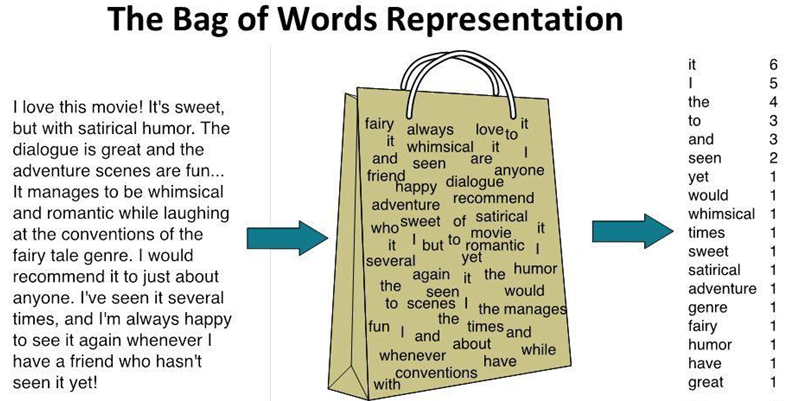
1f11cfef491e4c878f4b16bc791dcb75

Figure: Bag-of-words representation.

The early applications of machine learning in NLP relied on bag-of-words models. Modern applications, especially those related to Large Language Models, rely predominantly on sequence models.

18.5 Sequence Models Approach¶

Sequence models preserve the order of words in the input text. Typical implementation of sequence models includes representing the words in text data with integer indices, mapping the integers to vector representations, and passing the vectors to a machine learning model, where the layers in the model will account for the ordering of input vectors.

The input vectors to sequence models can be in the form of:

One-hot word vector representation, or
Word embeddings representation.

One-Hot Word Vector Representation¶

One-hot word vector representation is similar to encoding categorical features with one-hot encoding matrix. That is, the index for each word is converted to one-hot vector, having 1 (hot) for that word and 0 (cold) for all other words. An example is shown in the left-hand figure, where we created a zero vector with length of 4, and assigned 1 for the index that corresponds to every word. Another example is shown in the right-hand figure.

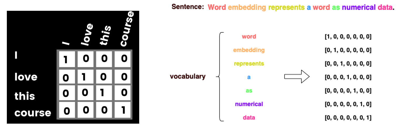
ee5dffe2334f4aea81e706f96c28ab08

Figure: One-hot word vector encoding.

One-hot word vector representation is not an efficient way to represent text, because for large text datasets the input vectors can become quite large. For instance, a training set with 20,000 words will need to use one-hot vectors of size 20,000 to represent each word, and this results in slow training, as well as this type of word representation takes a lot of memory space.

Using word embeddings is more efficient, since the vectors for word representation are much smaller than the size of the vocabulary, and more importantly, embedding vectors can capture important semantic meaning of the words. Hence, most modern NLP models rely on word embeddings for representing words in text.

18.5.1 Word Embeddings¶

Word embeddings representation is used to convert each word into a vector (also referred to as embedding vector), in such as way that the embedding vectors of words that have similar semantic meaning have close spatial positions in the embeddings space.

The embeddings space consists of the set of vectors, where each word in the vocabulary is represented with one vector. For calculating the distance between the vectors in the embeddings space, typically cosine similarity is used as a distance metric. For two vectors $u$ and $v$, cosine similarity is calculated as the dot (scalar, inner) product of the vectors divided by the norm of the vectors, i.e., $\dfrac{u\cdot v}{||u||\cdot ||v||}$.

Typical dimensionality of vectors for representing word embeddings in NLP models has been between 256 and 1,024. In modern LLMs, the dimensionality of token embeddings is commonly between 2,048 and 7,168. For instance, the following figure shows the embedding vector for the word ‘work’. The embedding vector has many values, and each value represents some aspect of the meaning of that word.

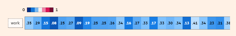
e2a39afe7be54a43a4d41ceeb1c65de4

Figure: Embedding vector for the word ‘work’. Source: link

The embedding vectors of words that have similar meanings are also similar. In the following figure, we can see that the embedding vectors of the words ‘football’ and ‘soccer’ are more similar to each other, than the embedding vectors of the words ‘sea’ or ‘we’.

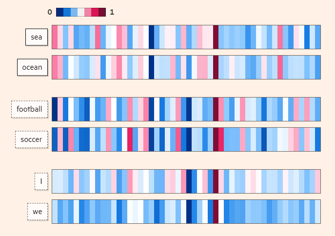
49327e1aae1f4b2fab67c43261b48280

Figure: Embedding vectors for words with similar meanings are also similar. Source: link

A simple example of word embeddings space is shown below, where similar words are positioned closer to each other. Therefore, the spatial distance between the vectors is dependent on the semantic meaning of the words.

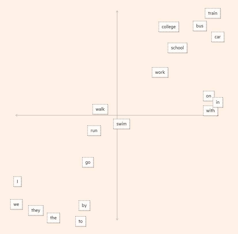
00aea5a43e124cf09b7a55939bbd5d06

Figure: Word embeddings space. Source: link

Two popular methods for generating word embeddings are word2vec and GloVe. These methods use Neural Networks to learn embedding vectors from a large corpus of text. The resulting vectors learned by these techniques can be imported as pretrained word embeddings and applied to downstream tasks with smaller training datasets.

For example, the website Embedding Projector provides visualizations of word embeddings, and for an entered word displays other words that are adjacent in the embeddings space.

To demonstrate the use of word embeddings with TensorFlow-Keras, we will implement it for a sentiment analysis task, to classify movie reviews using the IMDB Reviews dataset.

Loading the IMDB Reviews Dataset¶

IMDB Reviews Dataset can be downloaded from the built-in datasets in TensorFlow-Keras. There are 25,000 samples of movie reviews for training and 25,000 samples for validation. Setting max_features to 20,000 means we are only considering the first 20,000 words and the rest of the words will have the out-of-vocabulary token. Each movie review has a positive or negative label.

The training and validation datasets will be loaded as lists with 25,000 elements.

[ ]:

max_features = 20000

(train_data, train_labels), (val_data, val_labels) = tf.keras.datasets.imdb.load_data(num_words=max_features)

[ ]:

print(len(train_data))
print(len(val_data))

25000
25000

Displayed below is one example of a movie review. It is a list of indices, it contains 141 words, and as we can see the words in the dataset are already converted to integer indices.

[ ]:

# Display the third movie review
print('Number of words in the third review', len(train_data[2]))
print(train_data[2])

Number of words in the third review 141
[1, 14, 47, 8, 30, 31, 7, 4, 249, 108, 7, 4, 5974, 54, 61, 369, 13, 71, 149, 14, 22, 112, 4, 2401, 311, 12, 16, 3711, 33, 75, 43, 1829, 296, 4, 86, 320, 35, 534, 19, 263, 4821, 1301, 4, 1873, 33, 89, 78, 12, 66, 16, 4, 360, 7, 4, 58, 316, 334, 11, 4, 1716, 43, 645, 662, 8, 257, 85, 1200, 42, 1228, 2578, 83, 68, 3912, 15, 36, 165, 1539, 278, 36, 69, 2, 780, 8, 106, 14, 6905, 1338, 18, 6, 22, 12, 215, 28, 610, 40, 6, 87, 326, 23, 2300, 21, 23, 22, 12, 272, 40, 57, 31, 11, 4, 22, 47, 6, 2307, 51, 9, 170, 23, 595, 116, 595, 1352, 13, 191, 79, 638, 89, 2, 14, 9, 8, 106, 607, 624, 35, 534, 6, 227, 7, 129, 113]

[ ]:

# Display the first 10 train labels
train_labels[:10]

array([1, 0, 0, 1, 0, 0, 1, 0, 1, 0])

Preparing the Dataset¶

Let’s pad the data using the pad_sequences function in TensorFlow-Keras. Setting maxlen indicates to use the first 200 words in each movie review, and ignore the rest. Most movie reviews in the dataset are shorter than 200 words, however for those that are longer than 200 words some information will be lost. That is a tradeoff between computational expense and model performance.

[ ]:

train_data = pad_sequences(train_data, maxlen=200)
val_data = pad_sequences(val_data, maxlen=200)

[ ]:

# Print the shape of the padded train dataset
print('Shape of the train data:', train_data.shape)

Shape of the train data: (25000, 200)

We can see in the next cell that for the third review, which has a length of 141 words, the first 59 words are now 0, and the length is 200.

[ ]:

# Display the third movie review
print(train_data[2])

[   0    0    0    0    0    0    0    0    0    0    0    0    0    0
    0    0    0    0    0    0    0    0    0    0    0    0    0    0
    0    0    0    0    0    0    0    0    0    0    0    0    0    0
    0    0    0    0    0    0    0    0    0    0    0    0    0    0
    0    0    0    1   14   47    8   30   31    7    4  249  108    7
    4 5974   54   61  369   13   71  149   14   22  112    4 2401  311
   12   16 3711   33   75   43 1829  296    4   86  320   35  534   19
  263 4821 1301    4 1873   33   89   78   12   66   16    4  360    7
    4   58  316  334   11    4 1716   43  645  662    8  257   85 1200
   42 1228 2578   83   68 3912   15   36  165 1539  278   36   69    2
  780    8  106   14 6905 1338   18    6   22   12  215   28  610   40
    6   87  326   23 2300   21   23   22   12  272   40   57   31   11
    4   22   47    6 2307   51    9  170   23  595  116  595 1352   13
  191   79  638   89    2   14    9    8  106  607  624   35  534    6
  227    7  129  113]

Embedding Layer in TensorFlow-Keras¶

TensorFlow-Keras has Embedding layer, which we will use to project the input tokens into vectors in an embedding space. The Embedding layer requires at the minimum to specify the number of tokens in the data sequences, and the dimensionality of the vectors in the embeddings space. The layer takes integer indices as inputs, and outputs embedding vectors. It can be considered as a look-up table, which maps each integer index to an embedding vector.

To understand how the Embedding layer works, let’s consider a dataset with the maximum number of words set to 100, and our aim is to represent the words with 5-dimensional vectors. In the cell below, the Embedding layer assigned random values to the list of indices 1, 2, and 3, and we can see that to each index a 5-dimensional vector is assigned. However, the embedding vectors are trainable, and when we include the Embedding layer in a model, as we train the model, words that are similar will get closer in the embeddings space.

[ ]:

from tensorflow.keras.layers import Embedding

# Embedding layer: represent a dataset with a vocabulary of 100 words with 5 dimensional vectors
embedding_layer = Embedding(input_dim=100, output_dim=5)

[ ]:

# Input layer: list [1, 2, 3] converted to TensorFlow tensor
input_layer = tf.convert_to_tensor([1, 2, 3])

# Inspect the input_layer
input_layer

<tf.Tensor: shape=(3,), dtype=int32, numpy=array([1, 2, 3], dtype=int32)>

[ ]:

# Apply the Embedding layer
output_layer = embedding_layer(input_layer)

# Print the embedding vectors
output_layer.numpy()

array([[-0.04237379,  0.04802616, -0.04056418, -0.04120548, -0.00101371],
       [ 0.02238672,  0.04152756, -0.02390041,  0.03987378,  0.02417493],
       [-0.00587286,  0.02061386, -0.00715909,  0.0491767 , -0.02104199]],
      dtype=float32)

Define, Compile, and Train the Model¶

Next, we will define a model that uses an Embedding layer to project the words in input sequences into 8-dimensional vectors. These vectors will be further processed through dense layers, and the last layer will predict the label of movie reviews. There are two labels: positive and negative movie review, therefore this is a binary classification problem.

[ ]:

from tensorflow.keras.layers import Input, Flatten, Dense, Dropout
from tensorflow.keras.models import Model

max_features = 20000   # Vocabulary size
embedding_dim = 8      # Embedding dimension

# Define the layers in the model
input_layer = Input(shape=(200,))
embedding_layer = Embedding(input_dim=max_features, output_dim=embedding_dim)(input_layer)
flatten_layer = Flatten()(embedding_layer)
dense_layer = Dense(32, activation='relu')(flatten_layer)
dropout_layer = Dropout(0.5)(dense_layer)
output_layer = Dense(1, activation='sigmoid')(dropout_layer)

# Create the model with inputs and outputs
model = Model(inputs=input_layer, outputs=output_layer)

We will compile the model with binary_crossentropy loss (two labels: positive and negative review) and adam optimizer.

[ ]:

model.compile(optimizer='adam', loss='binary_crossentropy', metrics=['accuracy'])

Before training the model, we can see the model summary.

[ ]:

model.summary()

Model: "functional"

┏━━━━━━━━━━━━━━━━━━━━━━━━━━━━━━━━━┳━━━━━━━━━━━━━━━━━━━━━━━━┳━━━━━━━━━━━━━━━┓
┃ Layer (type)                    ┃ Output Shape           ┃       Param # ┃
┡━━━━━━━━━━━━━━━━━━━━━━━━━━━━━━━━━╇━━━━━━━━━━━━━━━━━━━━━━━━╇━━━━━━━━━━━━━━━┩
│ input_layer (InputLayer)        │ (None, 200)            │             0 │
├─────────────────────────────────┼────────────────────────┼───────────────┤
│ embedding_1 (Embedding)         │ (None, 200, 8)         │       160,000 │
├─────────────────────────────────┼────────────────────────┼───────────────┤
│ flatten (Flatten)               │ (None, 1600)           │             0 │
├─────────────────────────────────┼────────────────────────┼───────────────┤
│ dense (Dense)                   │ (None, 32)             │        51,232 │
├─────────────────────────────────┼────────────────────────┼───────────────┤
│ dropout (Dropout)               │ (None, 32)             │             0 │
├─────────────────────────────────┼────────────────────────┼───────────────┤
│ dense_1 (Dense)                 │ (None, 1)              │            33 │
└─────────────────────────────────┴────────────────────────┴───────────────┘

 Total params: 211,265 (825.25 KB)

 Trainable params: 211,265 (825.25 KB)

 Non-trainable params: 0 (0.00 B)

[ ]:

history = model.fit(train_data, train_labels, validation_data=(val_data, val_labels), epochs=5)

Epoch 1/5
782/782 ━━━━━━━━━━━━━━━━━━━━ 8s 7ms/step - accuracy: 0.6360 - loss: 0.5894 - val_accuracy: 0.8681 - val_loss: 0.3075
Epoch 2/5
782/782 ━━━━━━━━━━━━━━━━━━━━ 3s 4ms/step - accuracy: 0.9160 - loss: 0.2284 - val_accuracy: 0.8614 - val_loss: 0.3275
Epoch 3/5
782/782 ━━━━━━━━━━━━━━━━━━━━ 3s 4ms/step - accuracy: 0.9686 - loss: 0.1046 - val_accuracy: 0.8553 - val_loss: 0.3994
Epoch 4/5
782/782 ━━━━━━━━━━━━━━━━━━━━ 4s 5ms/step - accuracy: 0.9888 - loss: 0.0461 - val_accuracy: 0.8473 - val_loss: 0.5096
Epoch 5/5
782/782 ━━━━━━━━━━━━━━━━━━━━ 3s 4ms/step - accuracy: 0.9938 - loss: 0.0237 - val_accuracy: 0.8492 - val_loss: 0.6085

18.5.2 Using TextVectorization Layer¶

TensorFlow-Keras also provides another way to preprocess text by using a TextVectorization layer, which can be included directly as a layer in Neural Networks to tokenize and vectorize text.

This layer performs the following preprocessing steps:

Standardize text by removing punctuation and lowering the text case.
Split sentences into individual tokens.
Convert the tokens into a numerical representation.

The functionality of TextVectorization is similar to the Tokenizer function in TensorFlow-Keras. However, unlike the Tokenizer function which is commonly used for preprocessing text before feeding it into a model, the TextVectorization layer can be directly integrated into a TensorFlow-Keras model, making it more suitable for end-to-end model pipelines.

The arguments in TextVectorization layer are:

max_tokens: maximum number of tokens in the vocabulary, where vocabulary is comprised of unique text units (words) in the data. E.g., if max_tokens=1000 the layer will only consider the 1000 most frequent tokens from the input text data when building the vocabulary.
standardize: denotes the standardization specifics to be applied to input data; by default, it is lower_and_strip_punctuation meaning to convert to lowercase and remove punctuation.
split: denotes what will be considered while splitting the input text; by default it is whitespace " ".
output_sequence_length: the length to which the sequences will be padded (if shorter than the length) or truncated (if longer than the length).

[ ]:

from tensorflow.keras.layers import TextVectorization

text_vect_layer = TextVectorization(max_tokens=1000, output_sequence_length=10)

[ ]:

# Sample sentences
sentences = ['TensorFlow is a deep learning library!',
             'Is TensorFlow powered by Keras API?']

The adapt() method is used to fit the sentences to the TextVectorization layer. The adapt() method will create a vocabulary of the most frequent tokens, and it will create a mapping from tokens to integer indices that will be used later for converting text into a numerical representation.

[ ]:

text_vect_layer.adapt(sentences)

[ ]:

# Vectorize the above sentences and display the output
vectorized_sentences = text_vect_layer(sentences)
print(vectorized_sentences)

tf.Tensor(
[[ 2  3 11  8  6  5  0  0  0  0]
 [ 3  2  4  9  7 10  0  0  0  0]], shape=(2, 10), dtype=int64)

[ ]:

# Get the vocabulary from the TextVectorization layer
vocab = text_vect_layer.get_vocabulary()

# Print each word and its corresponding index
for i, word in enumerate(vocab):
    print(f"{word}: {i}")

: 0
[UNK]: 1
tensorflow: 2
is: 3
powered: 4
library: 5
learning: 6
keras: 7
deep: 8
by: 9
api: 10
a: 11

Let’s pass a sample sentence to inspect the output.

[ ]:

sample_sentence = 'Tensorflow is a machine learning framework!'

vectorized_sentence = text_vect_layer([sample_sentence])

[ ]:

print('Original sentence:', sample_sentence)
print('Vectorized sentence:', vectorized_sentence)

Orginal sentence: Tensorflow is a machine learning framework!
Vectorized sentence: tf.Tensor([[ 2  3 11  1  6  1  0  0  0  0]], shape=(1, 10), dtype=int64)

Since the words 'machine' and 'framework' were not part of the sentences that we passed to the layer and hence are not in the vocabulary, they are both represented by 1 in the vectorized output, since the index 1 is reserved for words that are out of vocabulary (oov_token).

The output is padded with 0, and the length of the output sequence size is 10.

The TextVectorization layer performs all required text preprocessing steps at once, and another advantage of this layer is that it can be used inside a model.

18.5.3 Sequence Modeling with Recurrent Neural Networks¶

Recurrent Neural Networks (RNN) is a neural network architecture that is designed for handling sequential data. Examples of sequential data are time-series, texts (sequence of words or characters), audio (sequence of sound waves), video (sequences of images), genetic sequences (DNA sequence), etc.

Working with sequential data requires to preserve the sequence of the information flow in the data. For example, given the sentence Today, I took my cat for a [....], to predict the next word, there should be a way to capture and preserve the flow from the beginning to the end of the sequence.

In conventional feedforward networks (such as networks composed of fully-connected or convolutional layers), the information flows from the input layer to the output layer. Conversely, in RNNs, there is a feedback loop at each time step, which creates the recurrence. This is shown in the next figure, where at each time step of the RNN model, an input (e.g., word) is processed, then in the next step the succeeding word is processed based on the information from the previous word, etc. This way, the network can learn dependencies between words that are not adjacent.

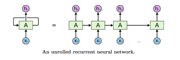
8413cafa5f704477a9466bf9a92876eb

Figure: Recurrent Neural Network.

There are three major types of RNN layers: conventional (a.k.a. basic, simple, vanilla) RNN, LSTM (Long Short-Term Memory), and GRU (Gated Recurrent Units). They are implemented in TensorFlow-Keras and PyTorch, and can be conveniently imported and used for creating models. In TensorFlow-Keras, the conventional (basic) RNN is called SimpleRNN, and LSTM and GRU are called as they are written.

While SimpleRNN has difficulty in handling long sequences, LSTM and GRU have the ability to store and preserve long-term dependencies over many time steps. Consequently, SimpleRNNs are rarely used at present.

Both LSTM and GRU layers use multiple gates to control the flow of information between the time steps. For instance, LSTM layers include an input gate and an output gate to control the input and output information for each time step, a forget gate that removes irrelevant information, and a memory cell that saves important information.

Next, we will apply an RNN model with LSTM layers for classification of text data.

Loading the Data¶

We are going to use the ag_news_subset dataset that is available in TensorFlow datasets. AG is a collection of news articles gathered from more than 2,000 news sources. The news articles are classified into 4 classes: World(0), Sports(1), Business(2), and Sci/Tech(3). The total number of training samples is 120,000 and testing 7,600.

Let’s get the dataset from TensorFlow datasets. In the load function, with_info=True will return various information about the dataset (as shown in the next cells), and as_supervised=True indicates that the data will be loaded as 2-element tuples consisting of (input, target) pairs.

[ ]:

import tensorflow_datasets as tfds
import pandas as pd

[ ]:

(train_data, val_data), info = tfds.load('ag_news_subset:1.0.0', #version 1.0.0
                                         split=['train', 'test'],
                                         with_info=True,
                                         as_supervised=True)

We can use info to check basic information about the dataset.

[ ]:

# Displaying the classes
class_names = info.features['label'].names
print(class_names)

['World', 'Sports', 'Business', 'Sci/Tech']

[ ]:

print('Number of training samples:', info.splits['train'].num_examples)
print('Number of validation samples:', info.splits['test'].num_examples)

Number of training samples: 120000
Number of validation samples: 7600

We can use tfds.as_dataframe to display the first 10 news articles as Pandas DataFrame.

[ ]:

news_df = tfds.as_dataframe(train_data.take(10), info)

news_df

	description	label
0	AMD #39;s new dual-core Opteron chip is designed mainly for corporate computing applications, including databases, Web services, and financial transactions.	3 (Sci/Tech)
1	Reuters - Major League Baseball\Monday announced a decision on the appeal filed by Chicago Cubs\pitcher Kerry Wood regarding a suspension stemming from an\incident earlier this season.	1 (Sports)
2	President Bush #39;s quot;revenue-neutral quot; tax reform needs losers to balance its winners, and people claiming the federal deduction for state and local taxes may be in administration planners #39; sights, news reports say.	2 (Business)
3	Britain will run out of leading scientists unless science education is improved, says Professor Colin Pillinger.	3 (Sci/Tech)
4	London, England (Sports Network) - England midfielder Steven Gerrard injured his groin late in Thursday #39;s training session, but is hopeful he will be ready for Saturday #39;s World Cup qualifier against Austria.	1 (Sports)
5	TOKYO - Sony Corp. is banking on the \$3 billion deal to acquire Hollywood studio Metro-Goldwyn-Mayer Inc...	0 (World)
6	Giant pandas may well prefer bamboo to laptops, but wireless technology is helping researchers in China in their efforts to protect the engandered animals living in the remote Wolong Nature Reserve.	3 (Sci/Tech)
7	VILNIUS, Lithuania - Lithuania #39;s main parties formed an alliance to try to keep a Russian-born tycoon and his populist promises out of the government in Sunday #39;s second round of parliamentary elections in this Baltic country.	0 (World)
8	Witnesses in the trial of a US soldier charged with abusing prisoners at Abu Ghraib have told the court that the CIA sometimes directed abuse and orders were received from military command to toughen interrogations.	0 (World)
9	Dan Olsen of Ponte Vedra Beach, Fla., shot a 7-under 65 Thursday to take a one-shot lead after two rounds of the PGA Tour qualifying tournament.	1 (Sports)

Now that we understand the data, let’s prepare it before we can use LSTMs to classify the news.

Preparing the Data¶

Note again that the variables train_data and val_data contain pairs of input text sequences and labels. First, we will separate the input text sequences and labels, and we will convert them to TensorFlow tensors with the convert_to_tensor function.

[ ]:

# Function to load the data as TensorFlow tensors
def load_data(dataset):
    inputs, labels = [], []
    for input_text, label in tfds.as_numpy(dataset):
        inputs.append(input_text)
        labels.append(label)
    return tf.convert_to_tensor(inputs, dtype=tf.string), tf.convert_to_tensor(labels)

# Load training and validation data directly as tensors
train_inputs, train_labels = load_data(train_data)
val_inputs, val_labels = load_data(val_data)

Let’s check the shape of the train and validation inputs and labels.

[ ]:

print("Training inputs shape:", train_inputs.shape)
print("Training labels shape:", train_labels.shape)
print("Validation inputs shape:", val_inputs.shape)
print("Validation labels shape:", val_labels.shape)

Training inputs shape: (120000,)
Training labels shape: (120000,)
Validation inputs shape: (7600,)
Validation labels shape: (7600,)

In the next cell, we can observe that the data type of the inputs is tf.string.

[ ]:

train_inputs.dtype

tf.string

To convert the text data into tokens, we will use the TextVectorizer layer in TensorFlow-Keras. Afterward, we will apply the adapt() method to preprocess the training data.

[ ]:

vocab_size = 20000

text_vect_layer = TextVectorization(max_tokens=vocab_size)

[ ]:

text_vect_layer.adapt(train_inputs)

Let’s pass two news articles to text_vect_layer. The vectorized sequences will be padded to the sentence with the maximum length, but if we wanted to have fixed size of padded sequences, we could set the output_sequence_length to another value in the layer initialization.

[ ]:

sample_news = ['This weekend there is a sport match between Man U and Fc Barcelona',
               'Tesla has unveiled its humanoid robot that appeared dancing during the show!']

[ ]:

vectorized_news = text_vect_layer(sample_news)
vectorized_news.numpy()

array([[   40,   491,   185,    16,     3,  1559,   560,   163,   362,
        13418,     7,  7381,  2517],
       [    1,    20,   878,    14,     1,  4663,    10,  1249, 11657,
          159,     2,   541,     0]])

Note that the second sentence was padded with 0. Also the words Tesla and humanoid have an index of 1 because they were not a part of the training data.

Creating and Training the Model¶

We are going to create a TensorFlow-Keras model that takes the sequences of text as input and outputs the class of the news articles.

The model has the following layers:

Input layer that takes input text sequences having tf.string type.
TextVectorization layer for converting input texts into tokens.
Embedding layer for representing the tokens with trainable embedding vectors. Because the embedding vectors are trainable, words that have similar semantic meaning will be represented by vectors that are close in the embeddings space.
LSTM layer for processing the sequences. The layer is wrapped into a Bidirectional layer, which will process the sequences from both directions (forward and backward), i.e., one LSTM layer will process the sequences forward, another layer will process the sequences backward, and the outputs of the two LSTMs will be combined.
Dense layer for classification purpose.

[ ]:

from tensorflow.keras.layers import Bidirectional, LSTM

embedding_dim = 64

# Define model layers
inputs = Input(shape=(1,), dtype=tf.string)
x = text_vect_layer(inputs)
x = Embedding(input_dim=vocab_size, output_dim=embedding_dim)(x)
x = Bidirectional(LSTM(64))(x)
x = Dense(64, activation='relu')(x)
outputs = Dense(4, activation='softmax')(x)

# Define the model
model = Model(inputs=inputs, outputs=outputs)

[ ]:

# Compile the model
model.compile(optimizer='adam', loss='sparse_categorical_crossentropy', metrics=['accuracy'])

[ ]:

# Train the model
history = model.fit(train_inputs, train_labels, validation_data=(val_inputs, val_labels), epochs=3, batch_size=32)

Epoch 1/3
3750/3750 ━━━━━━━━━━━━━━━━━━━━ 45s 11ms/step - accuracy: 0.8075 - loss: 0.5057 - val_accuracy: 0.9111 - val_loss: 0.2633
Epoch 2/3
3750/3750 ━━━━━━━━━━━━━━━━━━━━ 39s 10ms/step - accuracy: 0.9314 - loss: 0.2024 - val_accuracy: 0.9139 - val_loss: 0.2543
Epoch 3/3
3750/3750 ━━━━━━━━━━━━━━━━━━━━ 43s 11ms/step - accuracy: 0.9490 - loss: 0.1498 - val_accuracy: 0.9093 - val_loss: 0.2770

Let’s evaluate the model on news articles.

[ ]:

# Predicting the class of new news articles
sample_news_1 = tf.convert_to_tensor(['The self driving car company Tesla has unveiled its humanoid robot at a recent event!'])

# make predictions on the sample_news 1
predictions_1 = model.predict(sample_news_1)
print(predictions_1)

1/1 ━━━━━━━━━━━━━━━━━━━━ 0s 244ms/step
[[0.01865892 0.03239412 0.26387298 0.68507403]]

The model correctly predicted that the news article is related to tech or science.

[ ]:

# find the index of the predicted class
predicted_class_1 = np.argmax(predictions_1)

print('Predicted class:', predicted_class_1)
print('Predicted class name:', class_names[predicted_class_1])

Predicted class: 3
Predicted class name: Sci/Tech

One more example is provided in the next cell.

[ ]:

# Predicting the class of a new sample
sample_news_2 = tf.convert_to_tensor(['This weekend there is a match between two big footbal teams in the national league'])

predictions_2 = model.predict(sample_news_2)

predicted_class_2 = np.argmax(predictions_2)

print('Predicted class:', predicted_class_2)
print('Predicted class name:', class_names[predicted_class_2])

1/1 ━━━━━━━━━━━━━━━━━━━━ 0s 31ms/step
Predicted class: 1
Predicted class name: Sports

References¶

Complete Machine Learning Package, Jean de Dieu Nyandwi, available at: https://github.com/Nyandwi/machine_learning_complete.
Deep Learning with Python, Francois Chollet, Second Edition, Manning Publications, 2021.

BACK TO TOP